Instrumental Variables
- In practice, we rarely expect Assumption MLR.4 to hold for OLS.
- Problem of endogeneity: possible causes selection bias, reverse causality, measurement error, and many others.
- Instrumental Variables can solve failures of MLR.4. (sometimes)
Reference: Angrist and Pischke, Chapter 3, Wooldridge 15.1-15.2
Achievement Gap
Problem
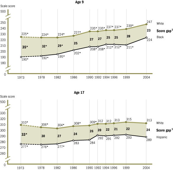
Black and Hispanic students score much lower on standardized tests compared to White and Asian students.
One potential reasons for this:
- Poor school quality in areas with large Black and Hispanic student population.
Are charter schools a solution?
Charter schools: publicly funded, independently operated schools.
Example: KIPP (Knowledge is Power Program) schools
- 88% students qualify for free lunch
- 95% students are Black or Hispanic

Treatment or Selection?
Minority students who go to KIPP schools score higher on standardized tests than minority students in public schools. But:
Is this a causal effect of KIPP schools? (Treatment effect)
Or is this because KIPP attracts different type of students (e.g. more intelligent, more motivated)? (Selection bias)
Model
$$ \text{Standarized test score} = \beta_0 + \beta_1 \text{KIPP attendance} + u $$
- Problem: KIPP attendance might be endogenous. Why? Students who attend KIPP might be more motivated, intelligent, ambitious, have more engaged parents, etc.
KIPP school in Lynn, MA was oversupscribed and offered seats with a random lottery.
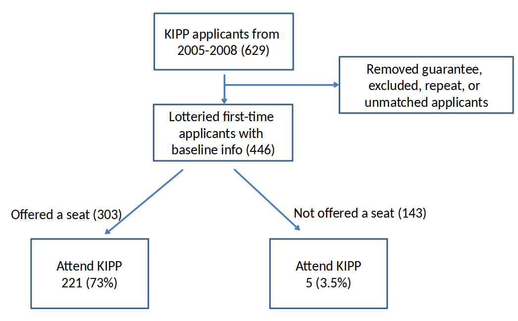
Offers were randomly assigned. Can we treat this as a randomized experiment?
Yes, we can estimate the causal effect of receiving an offer.
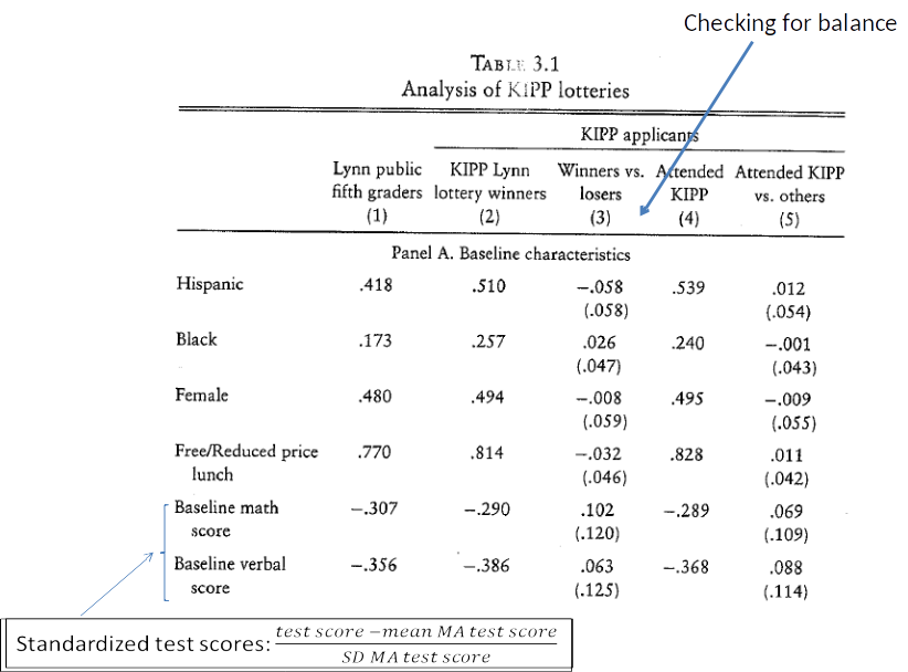
Note: Table 3.1 shows the standardized test score (mean = 0, SD = 1) in Math and Verbal.
Standardizing is done by subtracting the mean and dividing by the standard deviation for each test score.
This makes variables more easy to interpret:
A test score of 0 = mean score in the population
A test score of 1 = 1 SD above the mean

- But, only 73% student accepted the offer. Can we say something about the affect of attending KIPP Lynn?
- Do you the effect of attending KIPP Lynn will be larger or smaller than the effect of the receiving the offer?
From Offer to Attendance, intuition
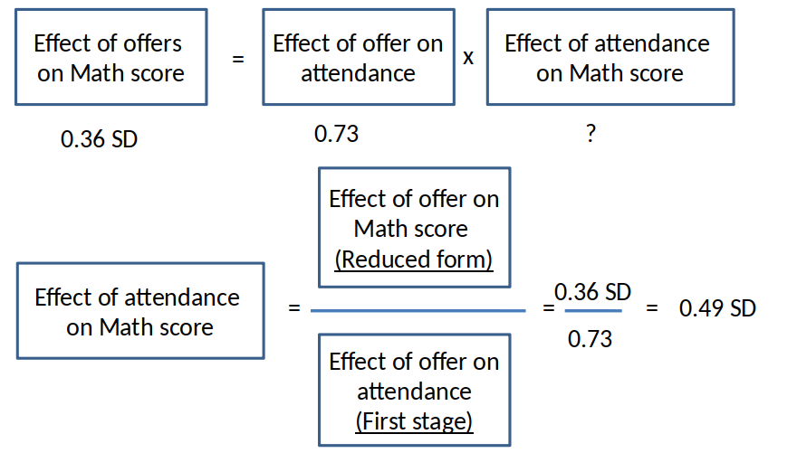
- IV estimate of causal effect is equal to the reduced form effect of the instrument, scaled up by the first stage. $$ \hat{\beta}_{IV} = \frac{\hat{\beta}_{RF}}{\hat{\beta}_{FS}} $$
Clicker question
What is the IV estimate of the effect of attending KIPP Lynn on Verbal score?
A) 0.15
B) 0.48
C) 0.61
D) Can’t say
IV in a simple regression framework
Consider this econometric model
$$ y=\beta_0 + \beta_1 x + u $$
We suspect that x and u are correlated, i.e. x is endogenous.
$$ Cov(x,u) \neq 0 $$
In this case OLS would lead to biased and inconsistent estimates of $\beta_1$.
The good news is that we can still get a consistent estimate of $\beta_1$ if we have a suitable instrumental variable.
IV Assumptions
In order to get consistent estimates of we need a variable $z$ that needs to fulfill the following conditions.
Instrument relevance: $Cov(z,x) \neq 0 $ z should be correlated with X.
Instrument exogeneity: $Cov(z,u) = 0 $. z should not be correlated with the error term.
IV Assumptions in the KIPP Example
$$ \text{Standarized test score} = \beta_0 + \beta_1 \text{KIPP attendance} + u $$
KIPP attendance might be endogenous
The instrument $z$ is the lottery status (win or lose).
Does the relevance assumption ($Cov(z,x) \neq 0$) hold?
Is lottery status correlated with KIPP attendance? Cov(lottery, attendance) $\neq 0$?Does the exogeneity assumption (Cov(z,u) $= 0$) hold?
Is the lottery status correlated with other factors that influence test score (u)? Cov(lottery, u) $= 0$?
Testing the IV relevance assumption
Recall from Chapter 2 that the slope estimator of a simple regression is $\hat{\beta}_1=\frac{Cov(x,y)}{Var(x)}$.
To test whether $Cov(z,x) \neq 0$ in the population we simply regress $x$ on $z$ in the sample.
If the coefficient is significantly different from zero we conclude that the relevance assumption holds.
In the KIPP example, we would run the following regression: $$ \widehat{attendance} = \hat{\beta_0} + \hat{\beta}_FS lottery $$
If $\hat{\beta}_{FS}$ is significantly different from zero, we conclude that the relevance assumption holds.
Testing the IV exogeneity assumption
- We cannot test the instrument exogeneity assumption $Cov(z,u) = 0$, because the error term $u$ is unobserved.
We have to argue that this is the case.
In the KIPP example, it is straightforward that if the lottery was random the lottery status ($z$) should be uncorrelated with all other factors that influence test score ($u$).
From assumptions to the IV estimator
instrument relevance $Cov(x,z) \neq 0$
instrument exogeneity $Cov(z,u) = 0$
Begin by studying the covariance between $z$ and $y$: $$ Cov(z,y)= Cov(z,\beta_0+\beta_1 x+u) $$ $$ Cov(z,y)= Cov(z,\beta_0)+ Cov(z,\beta_1 x) + Cov(z,u) $$ $$ Cov(z,y)= 0 + \beta_1 Cov(z,x) + Cov(z,u) $$
Under the IV assumptions (above), we can solve for $\beta_1$, $$ \beta_1 = \frac{Cov(z,y)}{Cov(z,x)} $$
From population to sample
$$ \beta_1 = \frac{Cov(z,y)}{Cov(z,x)} $$
Given a random sample, we can estimate $\beta_1$: $$ \hat{\beta}_1= \frac{\sum_{i=1}^{n} (z_i-\bar{z})(y_i-\bar{y})}{\sum_{i=1}^{n} (z_i-\bar{z})(x_i-\bar{x})} $$
This is the instrumental variables (IV) estimator of $\beta_1$.
IV = RF/FS
Recall that: $$ \hat{\beta}_{IV} = \frac{\hat{\beta}_{RF}}{\hat{\beta}_{FS}} $$
We know that $\hat{\beta}_{RF} = \frac{Cov(y,z)}{Var(z)} $ and $\hat{\beta}_{FS} = \frac{Cov(x,z)}{Var(z)} $
Plugging these into the equation above, it is straightforward to see that: $$ \hat{\beta}_{IV} = \frac{\frac{Cov(y,z)}{Var(z)}}{\frac{Cov(x,z)}{Var(z)}} = \frac{Cov(y,z)}{Cov(x,z)} $$
IV Variance
- The (asymptotic) variance of $\hat{\beta}_{IV}$ in the case with one endogenous variable and one instrument: $$ \frac{\sigma^2}{SST_x * R^2_{x,z}} $$ where is the R-squared of a regression of $x$ on $z$.
- Recall the variance of a simple OLS estimator: $$ \frac{\sigma^2}{SST_x} $$
- Since $R^2_{x,z}< 1$, IV variance will be larger than OLS variance. A stronger first stage implies a larger $R^2_{x,z}$ which leads to a smaller variance.
IV estimation in the regression framework
- The Two-stage least squares (2SLS) generalizes the IV estimate in a regression framework.
- Advantages:
- We can add control variables
- We can use multiple instruments
- We can easily implement it in Stata which automatically estimates correct standard errors
2SLS IV approach
Consider the econometric model $$ y = \beta_0 + \beta_1 x + \beta_2 c + u $$
- $x$: potentially endogenous variable of interest.
- $c$: exogenous control variable.
We suspect that $x$ and $u$ are correlated ($x$ is endogenous). $$ Cov(x,u) \neq 0$$
We have to make the same two assumptions,
- (15.5) $z$ is correlated with $x$: $Cov(z,x) \neq 0$.
- (15.4) $z$ is uncorrelated with $u$: $Cov(z,u) = 0$.
2SLS IV estimation, first stage
First stage: $$ x = \beta_{0,first} + \beta_{FS} z + \beta_{c,first} c + \upsilon $$
- Relevance assumption says that $Cov(z,x) \neq 0$. We can test this assumption by testing if $\beta_{FS}$ is significantly different from 0.
2SLS IV estimation, second stage
We then use the predicted values of $x$ from the first stage instead of $x$ in a regression on $y$.
Calculate predicted values of x: $$ \hat{x} = \hat{\beta}_{0,first} + \hat{\beta}_{FS} z + \hat{\beta}_{c,first} c $$
Second stage, regression: $$ y = \beta_0 + \beta_{FS} \hat{x} + \beta_c c + u $$
2SLS IV Estimation
- In practice, this procedure is easily implemented with Stata and other statistical software.
The statistical software also computes the correct standard errors.
Note that also in 2SLS estimation:
$$ \hat{\beta}_{2SLS} = \frac{\text{Reduced Form}}{\text{First Stage}} = \frac{\hat{\beta}_{RF}}{\hat{\beta}_{FS}} $$
Further points on IVs
If the relevance and exogeneity assumptions hold, the IV estimator is consistent but not unbiased.
(see topic 5, where we talked about consistency).Compared to OLS the IV estimator is less efficient (i.e., it has a larger variance, larger standard errors)
A stronger first stage leads to more efficient IV estimates.
(a strong instrument has high Cov(z,x))
Example 15.4 College proximity as an IV for education
Goal: Estimate the causal effect of education on wages, taking into account the possibility that education is an endogenous.
How: Use a dummy variable for whether someone grew up near a four-year colleage ($nearc4$) as an instrument for education.
First stage
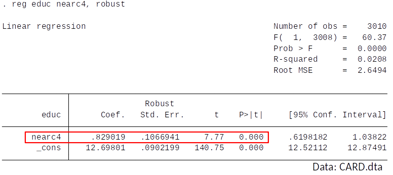
Is the instrument relevant? Is $Cov(educ,nearc4) \neq 0$?
Yes, college proximity significantly predicts years of education.
Reduced form
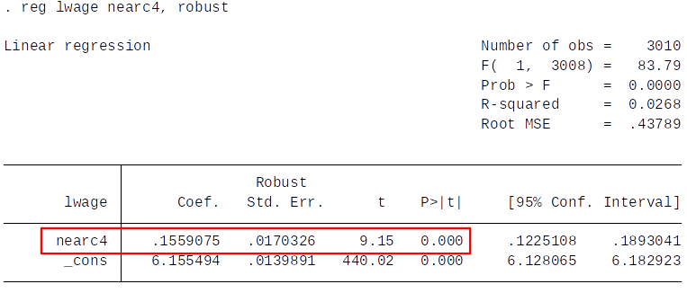
IV estimate of return to education: $$ \hat{\beta}_{2SLS} = \frac{\hat{\beta}_{RF}}{\hat{\beta}_{FS}} = \frac{0.156}{0.829} = 0.188 $$
IV estimation is very easily implemented using Stata:
Our IV estimate suggests that a one year increase in education leads to approx 19% increase in wage.
Stata automatically estimates the correct standard errors.
Is nearc4 exogenous?
Whether we should trust the IV estimates, depends on whether we believe the exogeneity assumption.
Is $Corr(nearc4, u) = 0$? (nearc4=distance to college; u=other factors that influence (log) wage)
Maybe people who live close to colleges have characteristics that make them earn more?
No problem if we can control for these factors.
2SLS is easily implemented in Stata
- ivregress 2sls
- You need to tell it what are $x$ and $z$.
- Stata automatically estimates the correct standard errors.
Estimated return to education: approx. 18%
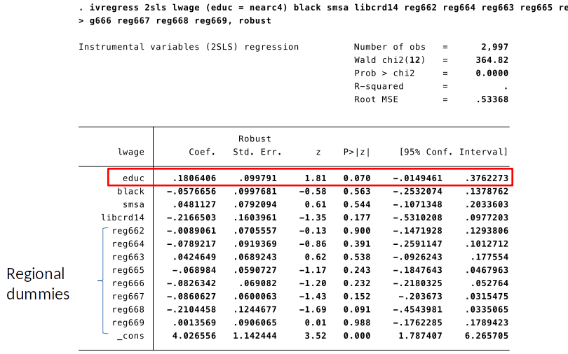
- Also when we include control variables, the 2SLS IV estimator is: $ \hat{\beta}_{2SLS} = \frac{\hat{\beta}_{RF}}{\hat{\beta}_{FS}} $
Interpretation of IV estimates
- So far we have (implicitly) assumed that is the same for all individuals.
- This is often not realistic.
- Is the return to education the same for all people?
- Will all students equally benefit from attending KIPP schools?
Let’s go back to the KIPP Lynn example:
Local Average Treatment Effect (LATE)
The effect estimated with IV is a Local Average Treatment Effect (LATE).
Local = only for those who are moved by the instrument
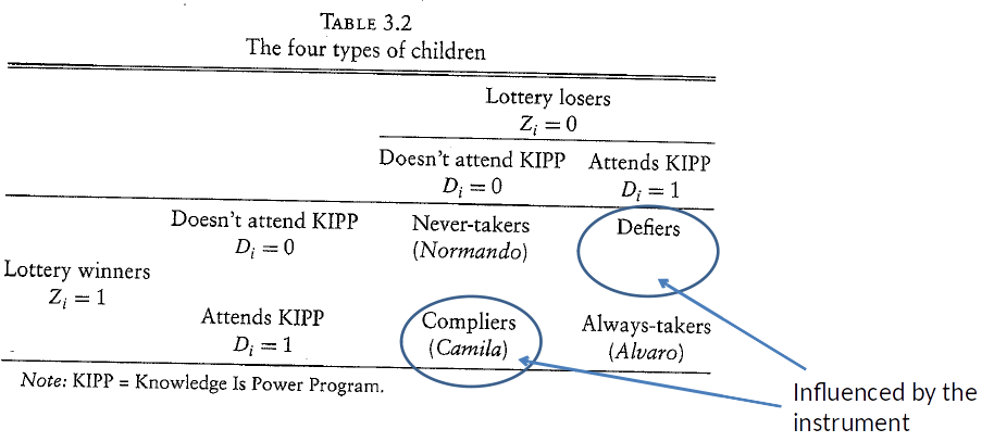
Local Average Treatment Effect = average treatment effect for those who were moved by the instrument (compliers + defiers).In the KIPP example, this means that IV estimates the average effect of going to KIPP on test scores for kids whose decision to go to KIPP was influenced by the lottery.
This means: causal effect might be different for never-takers and always-takers.
Average Treatment Effect (ATE)
- Recall: Monotonicity assumption: instrument influences the endogenous variable only in one direction (in our example: no defiers).
- If the monotonicity assumption holds (no defiers), LATE is the average treatment effect (ATE) for compliers.
Who is driving the estimates of return to education?
- IV estimates LATEs.
- Local: Who is moved by the instrument?
- People whose decision to go to college is influenced by the distance to college.
Are all of these moved in the same direction? Does the monotonicity assumption hold?
- Does college proximity only make people more and not less likely to go to college?
If yes, we have estimated of the average effect of education on wage for people who went to college because it is close, but wouldn’t have gone otherwise (compliers).
Summary
Instrumental variable estimation is a powerful and popular tool to get an estimate of a causal effects if $x$ is endogenous.
All we need is an instrumental variable that is correlated with $x$ (relevance assumption) and uncorrelated with $u$ (exogeneity assumption).
We can test the relevance assumption. We have to argue the exogeneity assumption.
IV is less efficient than OLS.
- IV estimates are LATEs.
Review/Other
Review IV: 1/2
Instrumental variable (IV) estimation is a powerful tool to estimate causal effects if OLS can’t.
All we need is an instrument $z$ that fulfils two assumptions:
- IV relevance: $Cov(z,x) \neq 0$
- $z$ should be correlated with $X$.
IV exogeneity: $Cov(z,u) = 0$.
- $z$ should not be correlated with the error term.
Review IV: 2/2
- We can test the IV relvance by regressing $X$ on $Z$ (first stage).
- We cannot test IV exogeneity, but have to think whether it is plausible.
- IV estimates are consistent but not unbiased.
- IV estimates are less efficient (have a larger variance) than OLS.