Pooled, Cross Section and Panel Data
- Types of Data
- Pooled OLS
- Difference-in-Difference Estimator
- First-Difference Estimator
Reference: Wooldridge, Chapter 1 and 13
Types of Data
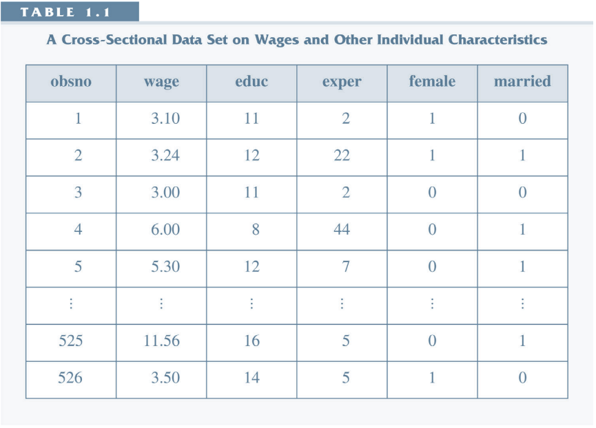
- Cross Section
- Many observations (individuals/households/firms etc.)
- Observed at one point in time.
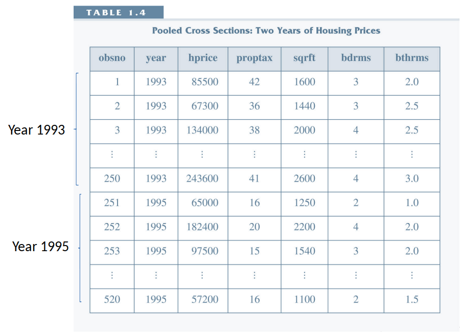
- Repeated Cross Section
- Many cross sectional datasets.
- Observed at different points in time (not the same observations).
- Pooled Cross Section: pool these repeated cross sections together and treat as one big cross section.
- Time Series (small n, large t)
- Few observation.
- Observed frequently.
- Panel Data (large n, small t)
- Many observations.
- Observed at few points in time.
Cross Section
- Everything we have seen so far is about cross-section.
- Lots of observations (large n)
- Observations (indexed by i) were assumed to be i.i.d: independent and identically distributed
Repeated Cross Section
- Multiple cross-sections.
- Loosely: observe groups of individuals at different time periods, but not the same individuals each time.
- (Still have the i.i.d assumption)
- We cannot follow an individual over time (cannot follow an individual from one cross section to another).
- But we can, e.g., look at how averages change over time.
Time Series
- Example: GDP observed every year.
- Small n (just one in above example), lots of time periods (indexed by t, large T).
- We expect GDP this year to be related to GDP last year.
- So we do not assume i.i.d.
- We might want to estimate things like: $y_t=\beta_0 + \beta_1 y_{t-1} + u$
- You can do this, but need to learn some new estimators/Econometrics. You cannot just use the exact same things we see in this course. You get the wrong answers if you do.
- We will not cover time series in this course. Be aware that you can do this, but that you need to go learn some new estimators to use for it. (They are not more difficult, just different.)
Panel Data
- Same individuals, observed in multiple time periods.
- Lots of individuals (large n, indexed by i), but only need a few time periods (small T, indexed by t).
- Important difference from repeated cross-section: same individuals in each time period.
- Now, we can look at how individuals change over time.
- With repeated cross-section we could only look at how averages change over time, not individuals.
Cross Section
Pooled Cross Section
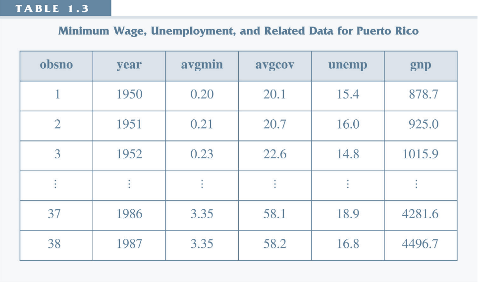
Time Series
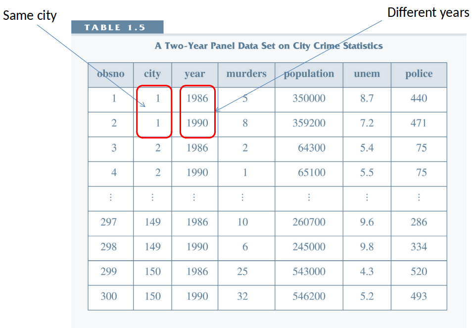
Panel Data
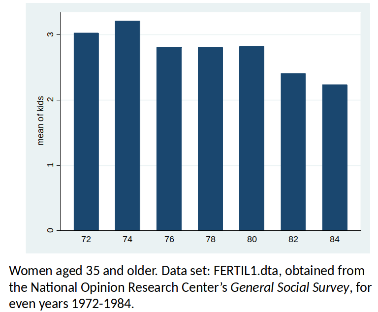
Women’s fertility (1972-1984), by year
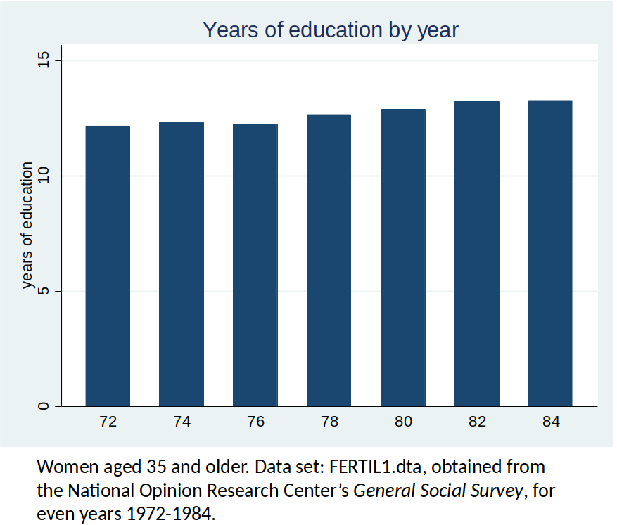
Women’s mean years of education (1972-1984), by year
Example 13.1
Women’s fertility over time
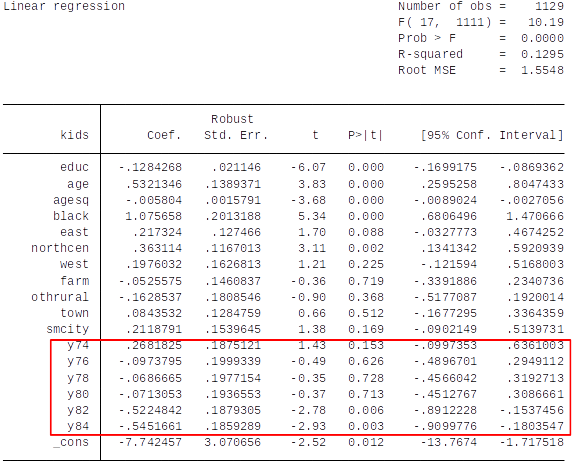
- Question: After controlling for other observable factors, what has happened to fertility rates over time?
- Dependent variable: kids, defined as the total number of kids born to a woman.
- Explanatory variables: education, age, race, region of the country where person lived at age 16, and living environment at age 16.
Pooled Cross Section.
- Pooling two or more independent cross sections is a straightforward extension of cross-sectional methods.
- Nothing new needs to be done in stating assumptions!
- The practically important issue is allowing for different intercepts, and possibly different slopes, across time.
Why might we want to pool cross sections?
- Larger sample size (=> lower standard errors)
- Enables us to estimate trends conditional on explanatory variables.
- Enables us to estimate how the effect of one factor has changed over time (e.g., how did the gender wage gap change?)
Interpretation of the Results
How should we interpret the coefficients on the year dummy variables? (Hint: First establish what is the base year – see lecture on dummy variables)
Are these estimated effects statistically and economically significant? Explain.
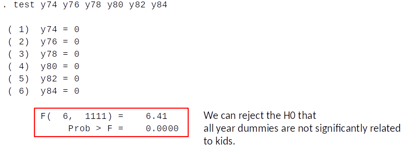
How would you test the null hypothesis that, conditional on the other explanatory variables (not related to time), fertility rates are constant over time?
How to test for significance of the results?
Test if year dummies jointly predict kids after controlling for educ, age, …?
We do an F-test:
- Remember from topic 6
- Intercepts might be different for different subgroups
- Slopes might be different for different subroups

With pooled cross section data we can find out if:
- The difference between subgroups changes over time
- The effect of a variable changes over time
We have data on two cross sectional datasets. One from 1978 and one from 1985.
- With this dataset we can answer these questions:
- Did the gender wage gap change from 1978 to 1985?
- Did the return to education change from 1978 to 1985?
- Did the gender wage gap change from 1978 to 1985?
- Did the return to education change from 1978 to 1985?
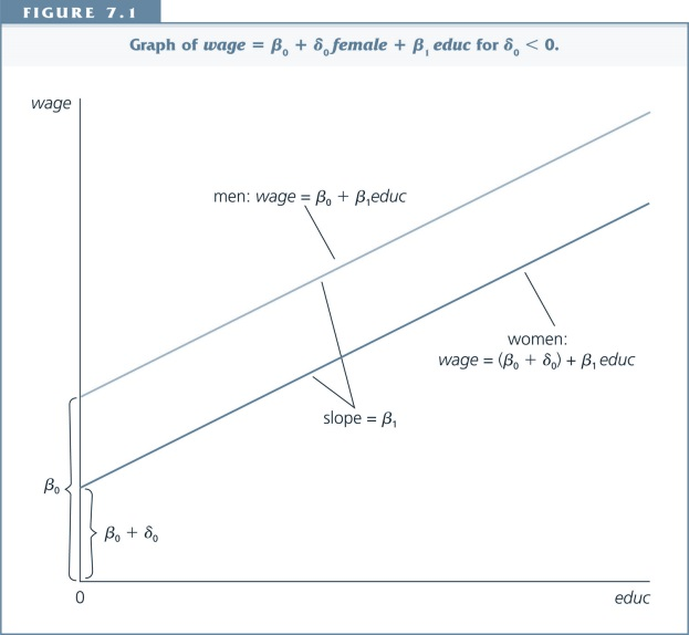
$$ ln(wage) = \beta_0 + \delta_0 y85 + \underbrace{\overbrace{\beta_1 educ}^{\text{Effect of education on wage in 1978: } \beta_1} + \delta_1 (y85*educ)}_{\text{Effect of education on wage in 1985: }\beta1+\delta_1} + \beta_2 exper \\ \quad \quad +\beta_3 exper^2 + \beta_4 union + \underbrace{\overbrace{\beta_5 female}^{\text{Effect of female on wage in 1978: }\beta_5} + \delta_5 (y85*female)}_{\text{Effect of female on wage in 1985: }\beta_5+\delta_5} + u $$
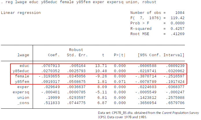
From 1978 to 1985: Estimated return to education increased from about 7% to about 10%
Estimated gender wage gap, conditional on education, experience, experience squared, Union, decreased from approx 32% to approx 23% (remember the approximation error discussed in topic 5)
What is the effect of building a refuse incinerator on housing prices?
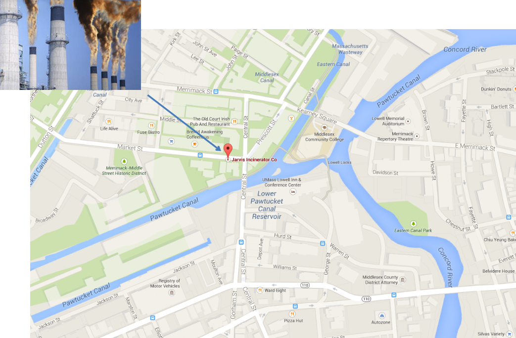
Background: A rumor that a new incinerator would be built in North Andover started after 1978; construction started in 1981.
We expect that the building of the incinerator has a negative effect on house prices.
Our simple econometric model is thus written as follows: $$ rprice=\beta_0 + \beta_1 nearinc + u $$
Where rprice is the house price in 1978 dollars, nearinc is a dummy variable equal to 1 if the house is near the incinerator and 0 otherwise.
We expect $\beta_1$ <0

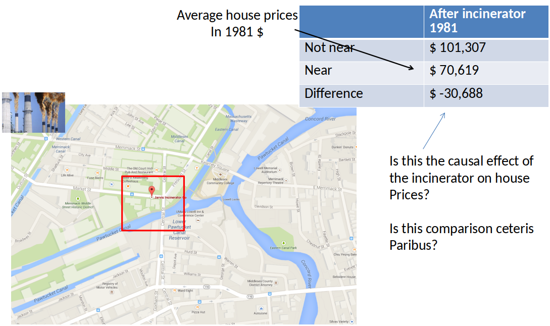
Price differences in 1981
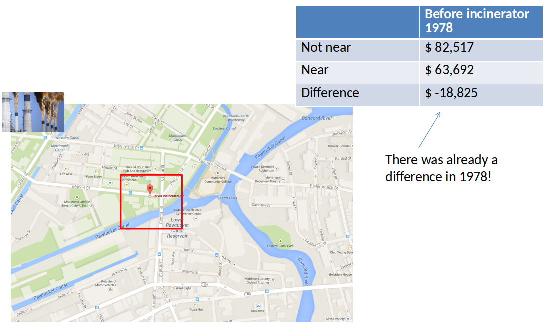
Price differences in 1978
Difference-in-Difference (Diff-in-Diff) estimator, intuition
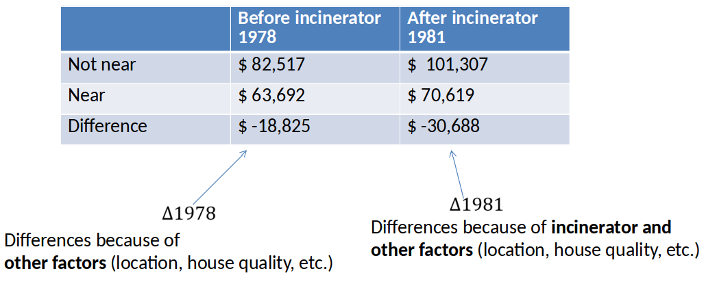
Diff-in-Diff estimator of effect of incinerator: $\Delta 1981 - \Delta 1978 = \$-11,863 $
- It is only valid if the difference due to the other factors is constant (unchanging) over time.
- Is \$-11,863 statistically significant? We can't tell from this table.
Graphical illustration of Diff-in-Diff
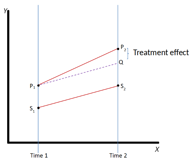
- Parallel trends assumption: The outcome of the treatment and control group would have followed a parallel trend in the absence of the treatment.
Parallel trends assumption
- Recall from topic 1:
causal effect of treatment = outcome if treated – outcome if not treated
Diff-in-Diff Estimation using OLS
We divide the observations into 2 groups:
- Control group: not affected by the policy change (houses far from the incinerator).
- Treatment group: affected by the policy change (houses near the incinerator).
We have 2 periods of data
- One year before the policy change.
- One year after the policy change.
We define 2 dummy variables:
- Treatment status dT (dT = 1 if Treatment group, dT = 0 if Control group)
- Time period d2 (d2 = 1 if after the policy change, d2 = 0 if before the policy change,)
We thus have four groups:
- Treatment group (dT=1), before the change (d2=0)
- Treatment group (dT=1), after the change (d2=1)
- Control group (dT=0), before the change (d2=0)
- Control group (dT=0), after the change (d2=1)
$$ y =\beta_0 + \delta_0 d2 + \beta_1 dT + \delta_1 \underbrace{(d2*dT)}_{\text{interaction term}} + u$$
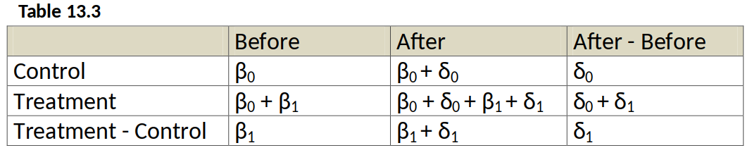
As long as there are no other explanatory variables in the regression, the OLS estimate of $\delta_1$ is numerically identical to $$ \hat{\delta}_1 = (\bar{y}_{2,T} - \bar{y}_{2,C}) - (\bar{y}_{1,T} - \bar{y}_{1,C}) $$ where $\bar{y}_{2,T}$ is the sample mean for the treated group in the period after the policy change (period 2), $\bar{y}_{1,C}$ is the sample mean for the control group before the policy change (period 1), and so on.
Diff-in-Diff in OLS framework $$ rprice = \beta_0 + \beta_1 nearinc + \beta_2 y81 + \beta_3 ( nearinc* y81) + u $$
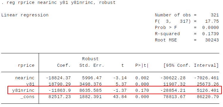
Should we reject the null hypothesis that the building of the incinerator did not cause lower house prices?
Adding Control Variables
There are 2 good reasons for adding control variables to a diff-in-diff model:
- The parallel trends assumption might be violated and we hope that the outcome conditional on the control variables would have followed a parallel trend for the treatment and control group. (i.e., that the control variables can fully account for/predict the deviations from parallel trends)
- Adding control variables can reduce the error variance and therefore the standard error of the diff-in-diff estimate.
Diff-in-Diff Estimation with Control Variables
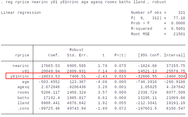
- How do these results compare to those obtained for the model without control variables? Discuss.
Example Diff-in-Diff by Marie & Zoelitz (2015)  
In Maastricht:
- Coffeeshops were open to everyone until September 2011
From October 2011 they were open only open for Dutch, Germans and Belgians (DGB) and closed for all other nationalities.
What is the effect of coffeeshop closing on academic performance?
(Coffeeshops is what the Dutch call places you can legally smoke weed)
Poster Announcing Application on 1st of October 2011

Course Grades for DGB and All Other Nationality Students
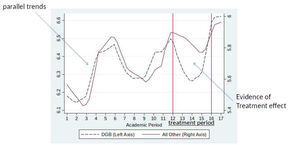
The performance of students who are no longer legally permitted to buy marijuana increases substantially.
This is evidence for causal effect of restricting access to marijuana on grades.
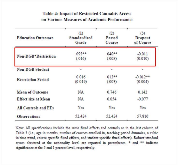
In a regression framework
They then estimated the following regression: $$ Y_{it} = \alpha + \beta_1 (NonDGB_i*Discrim_t) + \beta_2 NonDGB_i +\beta_3 Discrim_t + \epsilon_{it} $$
Where NonDGP is a dummy indicating if a student is not Dutch, German or Belgian.
- Discrim is a dummy equal to one for the discriminated period.
Results
What is the effect of unemployment on crime?

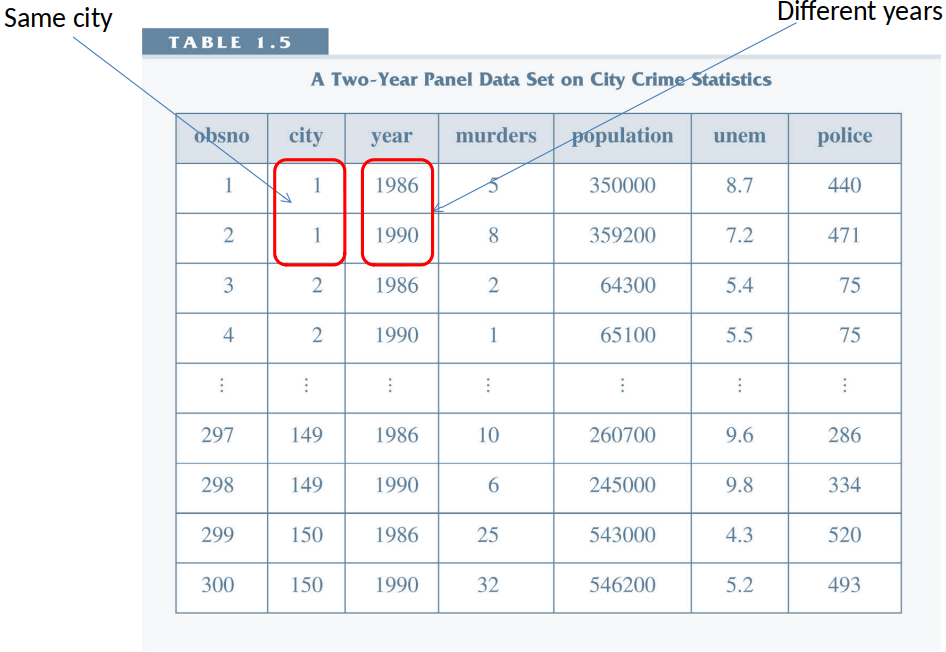
Data
CRIME2.dta: a panel data set on crime and unemployment rates for 46 cities for 1982 & 1987.
We observe each city twice!
Crmrte = crimes per 100,000 people
Unem = unemployment rate
y87 = year dummy (1 if year 1987)
Panel Data
Cross Section
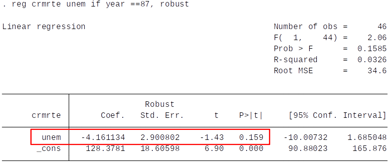
- High unemployment rate predicts low crime rates.
- Does this fit with what we might expect? There might be a problem with this specification due to omitted variables (e.g. geographical features).
Pooled Cross Section
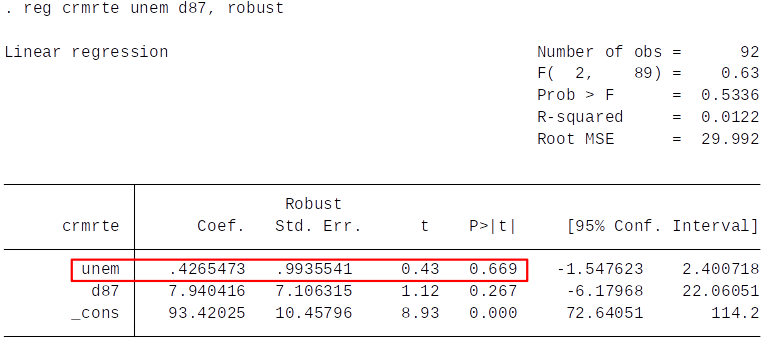
- More in line with our expectations, but there might still be omitted variable bias.
How would you weigh a dog that refuses to sit still on a scale?

First-Difference estimator, intuition
- By differencing every variable ($Y_2-Y_1$, $X_2-X_1$, etc.) we can relate changes in X to changes in Y.
- This allows us to hold time constant factors constant.
First Difference estimator, step by step
- Subscript $i$ denotes the cross-sectional unit (e.g., individual, city)
- Subscript $t$ denotes the time period (e.g., year, month)
We can then write a panel data model with a single observed explanatory variable as: $$ y_{it} = \beta_0 + \delta_2 period2_t + \beta_1 x_{it} + \upsilon_{it}, \quad \quad t=1,2$$
The error term $\upsilon_{it}$ can then be split up into:
- a time constant part $a_i$ (hence no time script)
- and a time varying part $u_{it}$
- That is, $\upsilon_{it}=a_i+u_{it}$
First Difference estimator, step by step
We can thus rewrite the model as follows: $$ y_{it} = \beta_0 + \delta_2 period2_t + \beta_1 x_{it} + a_i + u_{it}, \quad \quad t=1,2$$
$a_i$ is called a fixed effect.
- The error $u_{it}$ is often called the idiosyncratic (or time varying) error.
- The above model is often called the fixed effects model.
For each cross-sectional observation i, write the two years as, $$ y_{i2} = (\beta_0 + \delta_0) + \beta_1 x_{i2} + a_i + u_{i2}, \quad \quad t=2$$ $$ y_{i1} = \beta_0 + \beta_1 x_{i1} + a_i + u_{i1}, \quad \quad t=1$$ Next, subtract the second equation from the first, $$ (y_{i2}-y_{i1}) = \beta_0 + \beta_1 (x_{i2}-x_{i1}) + (u_{i2}-u_{i1}), \quad \quad t=1$$ $$ \Delta y_{i2} = \delta_0 + \beta_1 \Delta x_{i2} + \Delta u_{i2} $$
$a_i$ has been differenced away, so what?
$$ \Delta y_{it} = \delta_0 + \beta_1 \Delta x_{it} + \Delta u_{it} \quad \quad \quad \quad \quad \text{(Equation 13.17)} $$
- The good news: Even if $a_i$ is correlated with $x_it$, we may obtain an unbiased estimate of $\beta_1$.
- Equation (13.17) is called a first-differenced equation and we can simply estimate it with OLS.
- We need to consider the OLS assumptions as before.
- We can now write assumption SLR. 4 as follows:
- $u_{it}$ must be uncorrelated with the explanatory variable in both periods.
First Differenced Data in Stata
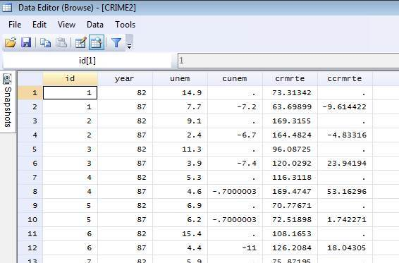
Cunem = change in unemployment rate (unemployment rate in 87 – unemployment rate rate in 82).
Ccrmrte = change in crime rate (crime rate in 87 – crime rate in 82)
Example: crime rate and unemployment
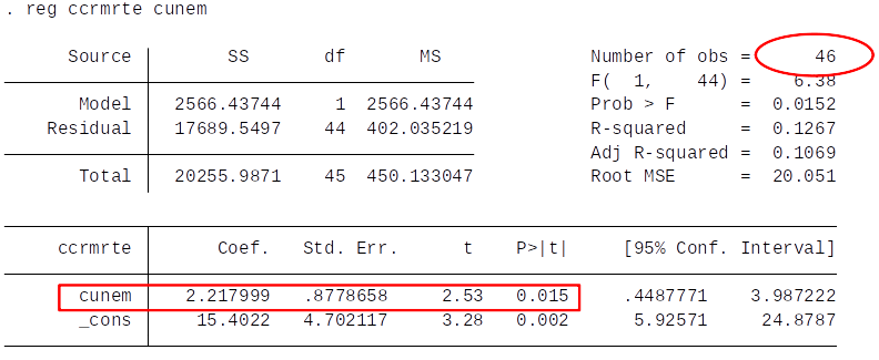
FD estimates predicts that if unemployment rate increases by 1 percentage point Crime rate increases by 2.217 (per 100,000 population)
- Whether our estimator is unbiased depends on SLR.4: $$ E(\Delta u_{it} | \Delta unemployment_{it} ) = E(\Delta u_{it})$$
- Could there be time varying factors that are correlated with crime?
- What if cities start hiring more police when the unemployment rate decreases?
- Hiring police might be a mechanism.
- What if a change in Government affects both crime and unemployment?
- As long as we can control for changes in Government we are fine.
Clicker question
The pooled OLS estimate of the effect of area (in square mile) on crime rate is 0.0031. What do you think is the First-Difference OLS estimate of area (in square mile) on crime rate?
A) 0.056
B) -0.024
C) 0.325
D) Can’t say/Not defined
Keep in Mind
- Differencing the two years of panel data is a powerful way to control for unobserved (time-constant) effects.
BUT:
- Panel data sets are harder to collect than a single cross section
- The differencing used to eliminate $a_i$ can greatly reduce the variation in the explanatory variables; that is, while $x_{it}$ may have a lot of variation, $\Delta x_{it}$ may not. One implication would be a large standard error (why?).
- If $x_{it}$ changes little or not at all over time (e.g., years of education amongst adult workers), then the above approach will not work well in practice.
Example: Effect of receiving a training grant on productivity
- The government gives out training-grants to firms who apply.
- Grants are awarded on a first-come first serve basis (grant = 1 if firm received a grant).
A measure of productivity is the scrap rate (scrap) (defect items per 100).
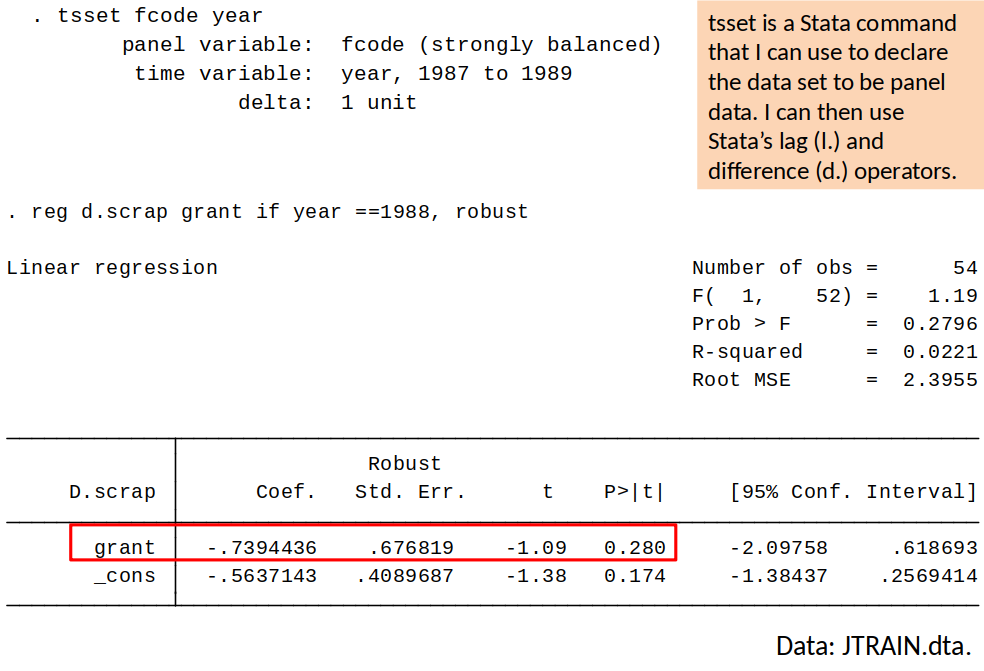
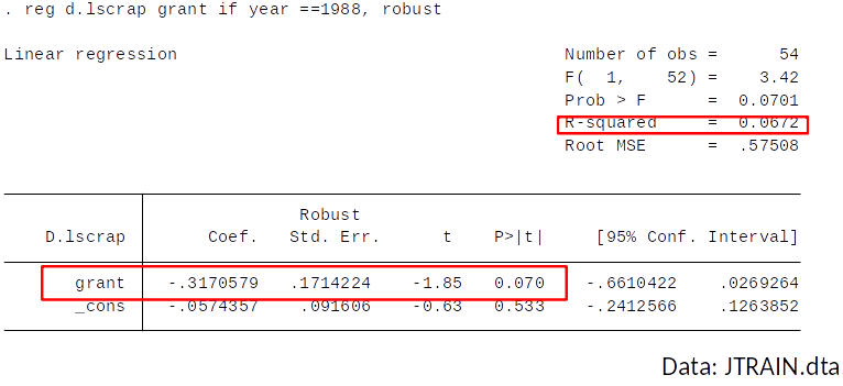
Model: $$ scrap_{it} = \beta_0 + \delta_0 d88_t + \beta_1 grant_{it} + a_i + u_{it} $$
$$ scrap_{it} = \beta_0 + \delta_0 d88_t + \beta_1 grant_{it} + a_i + u_{it} $$
Years: 1987 and 1988.
- What factors might be captured by the term $a_i$?
- Why might $a_i$ be correlated with whether a firm receives a grant?
Differencing to remove $a_i$ gives: $$ \Delta scrap_{it} = \delta_0 + \beta_1 \Delta grant_{it} + u_{it} $$
Therfore, we simply regress the change in the scrap rate on the change in the grant indicator.
Note that, since no firm received a grant in 1987, the change in the grant indicator is equal to the indicator for whether the firm received a grant in 1988.