Dummy Variables
- Incorporate qualitative information.
- Different effects for different groups.
Reference: Wooldridge, Chapter 7
Qualitative Information
- What is the effect of being female on wage?

- As long as we can put qualitative information into categories we can estimate their effect using OLS.
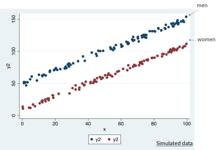
Is the OLS regression line a good description of the data?
Express categories in terms of dummy variables
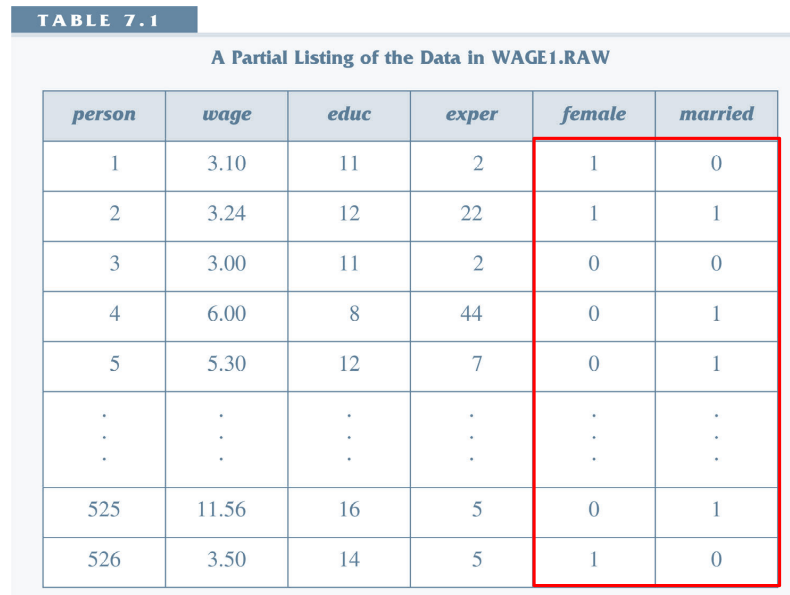
We can express belonging to a certain category with a binary indicator:
1 = belonging to a category
0 = not belonging to a categoryExample: We can express female as a dummy variable by assigning the value 1 for all females and 0 to all others.
You can transform any information into a dummy variable. It is totally arbitrary.
DHigh = 1 if individual is educated more than 12 years, 0 if individual is educated less than 12 years
Data with dummy variables
Incorporating Dummys in DGPs
We can then express the effect of being in a category by simply including it in the DGP.
The effect of being female on wage can be expressed as follows, $$ wage = \beta_0 + \delta_0 female + u $$
$\delta_0$ captures the effect of being female on wage.
Base Group
The base group (reference group/comparison group) is the group against which we compare the effect of the dummy variable. $$ wage = \beta_0 + \delta_0 female + u $$
In this example, the base group is males$^*$. Thus, $\delta_0$ shows the effect of being female compared to being male on wage.
$*$: We will assume for this exercise that the dataset only consists of males and females. If it contained other genders, the base group would be males and all other genders.
Example wage equation
- Imagine the wage equation with a dummy variable indicating whether an invidividual is female, $$ wage = \beta_0 + \delta_0 female + \beta_1 educ + u $$
Recall that $female$ takes value 1 for women, 0 for men.
When $female=1$ (i.e., for women), get $$ wage = \underbrace{\beta_0 + \delta_0}_{intercept} + \beta_1 educ + u $$
When $female=0$ (i.e., for men), get $$ wage = \underbrace{\beta_0}_{intercept} + \beta_1 educ + u $$
Note the difference between the two equations is $\delta_0$ which generates a shift in the intercept.
Example 7.1: Gender Wage Gap
- Let us calculate the sample descriptive statistics, i.e., some mean values of the variables.
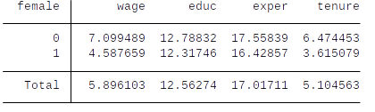
- The average hourly wage of males is \$7.10 and it is \$4.59 for females. The raw (unconditional) wage difference between females and males is \$2.51
- Note that this difference is not ceteris paribus and males and females differ for example in terms of educ, exper and tenure.
- Imagine we want to estimate the following model: $$ wage = \beta_0 + \delta_0 female + u $$
- An wage regression where we only include the female dummy will also give us the average wage difference:
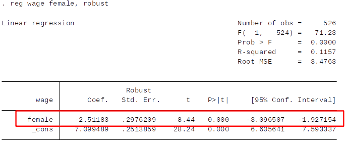
- is exactly -\$2.51 and the intercept is \$7.10. It is clear that:
- When female = 0, the predicted wage is the wage of males: 7.10
- When female = 1, the predicted wage is the wage of females : 7.10- 2.51 = 4.59
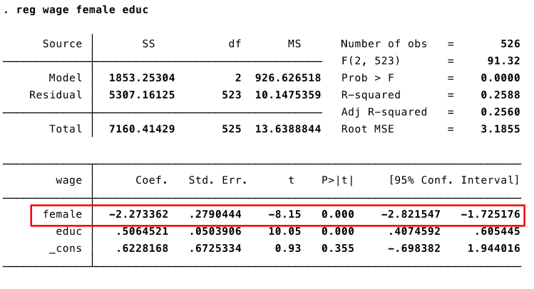
Let's estimate the following model: $ wage = \beta_0 + \delta_0 female + \beta_1 educ + u $
Switching the base group
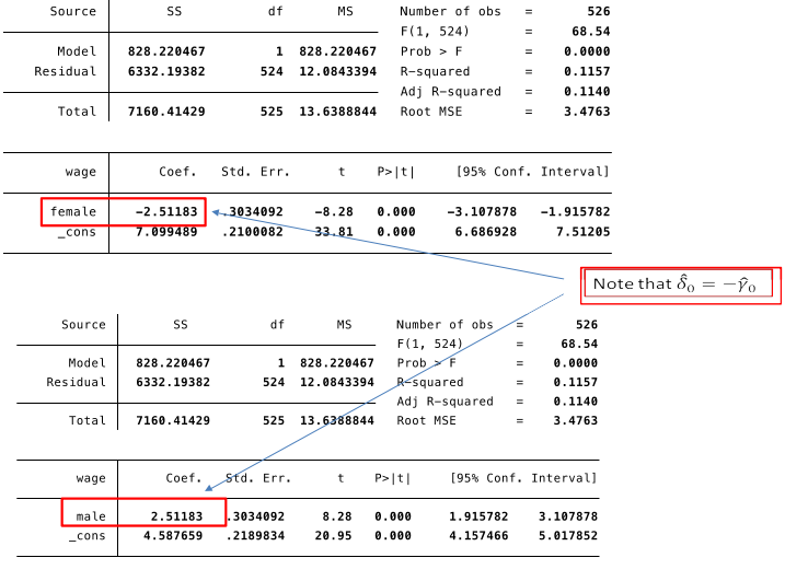
Old specification of the DGP: $ wage = \beta_0 + \delta_0 female + u $
We could instead specify the model DGP as: $ wage = \beta_0 + \gamma_0 male + u $
where $male$ is a dummy variable equal to $1$ if the individual is male and $0$ if the individual is female.- $\gamma_0$ is thus the effect of being male compared with being female on wages.
- Note that this means that $\gamma_0=-\delta_0$.
- Which group you choose as the base group makes no mathematical difference. It only matters for how you interpret the coefficient.
Dummy Variable Trap
- Why not include two dummy variable, one each for females and males ? $$ wage = \beta_0 + \delta_0 female + \gamma_0 male + \beta_1 educ + u $$
- You cannot do this when there is a intercept in the model. Why?
It generates a perfect colinearity (MLR 3). You can perfectly predict male from female and vice versa. This is called dummy variable trap.
Stata will automatically drop one of the redundant dummy variables
Dummy Variables with Multiple Categories
In practice you may have qualitative variables with more than two categories.
In this case we create more than one dummy variable: one for each category.
In the regression, we have to leave one of these dummy variables out which will be the base group.
Example: Dummies for different Marital Statuses
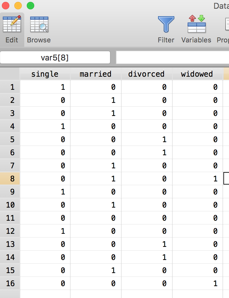
Let’s say we want to distinguish between four marital statuses:
Single, married, divorced and widowed.
We can then create a a dummy variable for each category.
E.g.: $single$ = 1 if person is single and 0 otherwise (i.e., if married, divorced or widowed)
Dummy variables for ordinal categories
An ordinal variable, is a variable where the order matters but not the difference between values.
E.g., $raceresult$ which takes values of 1 for first, 2 for second, 3 for third, et cetera. (there is an ordering, but no reason to think the difference between 1st and 2nd place is same as between 2nd and 3rd place).We can estimate the effect of an ordinal variables by creating a dummy for each category.
We then again include all of them except one (the base group) in the regression.
The coefficient on the dummy variable can then be interpreted as effect compared to the base group.
What not to do: What goes wrong if we create a variable $maritalstatus$ which takes values of 0 for $single$, 1 for $married$, 2 for $divorced$ and 3 for $widowed$ and simply put that in our regression? (Hint: Why would you expect the effect of $divorced$ to be double the effect of $married$? Why would you expect difference between effect of $widowed$ and $divorced$ to be the same as the difference between $married$ and $single$?)
Example: Effect of Physical Attractiveness on Wage
Hamermesh and Biddle (1994) estimate the effect of physical attractiveness on wage.
They use ratings on the beauty using 3 categories (below average, average, above average).
The order of the rating is clear (above average > average> below average), but the difference is not (above average = 2 * average ????)
They therefore include a dummy for above average (1 if beauty is above average, else 0) and a dummy for below average (1 if beauty is below average, else 0).
The base group is average.
Let's estimate the following model: $wage=\beta_0 + \beta_1 belavg + \beta_2 abvavg + u$
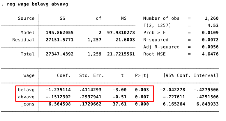
- Below average looking people earn \$1.23 less per hour compared to average looking people (base group).
- Above average looking people earn about the same per hour compared to average looking people (base group).
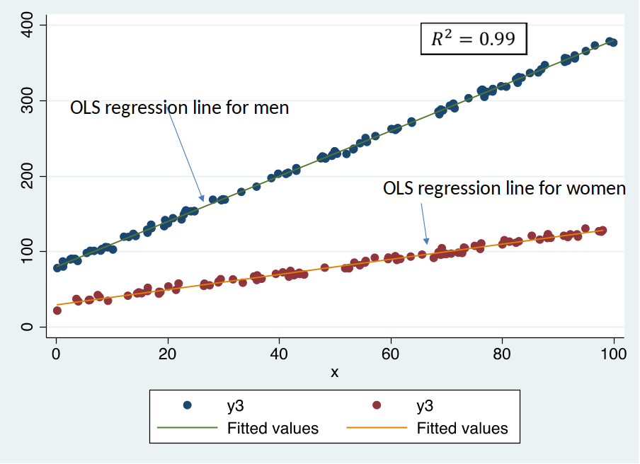
Different effects for different subgroups
- What is the return to education for men vs women?
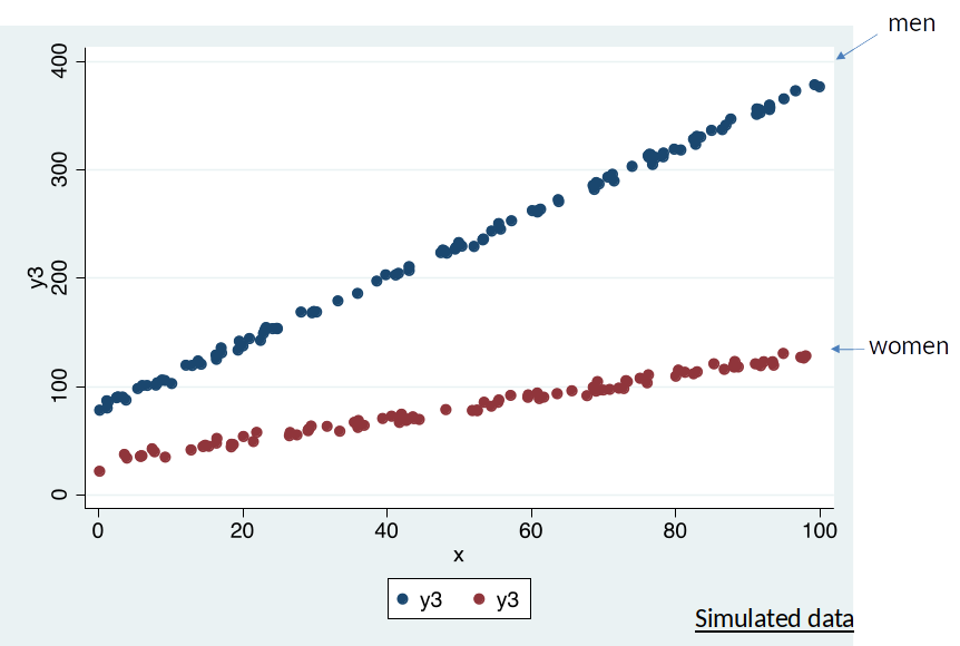
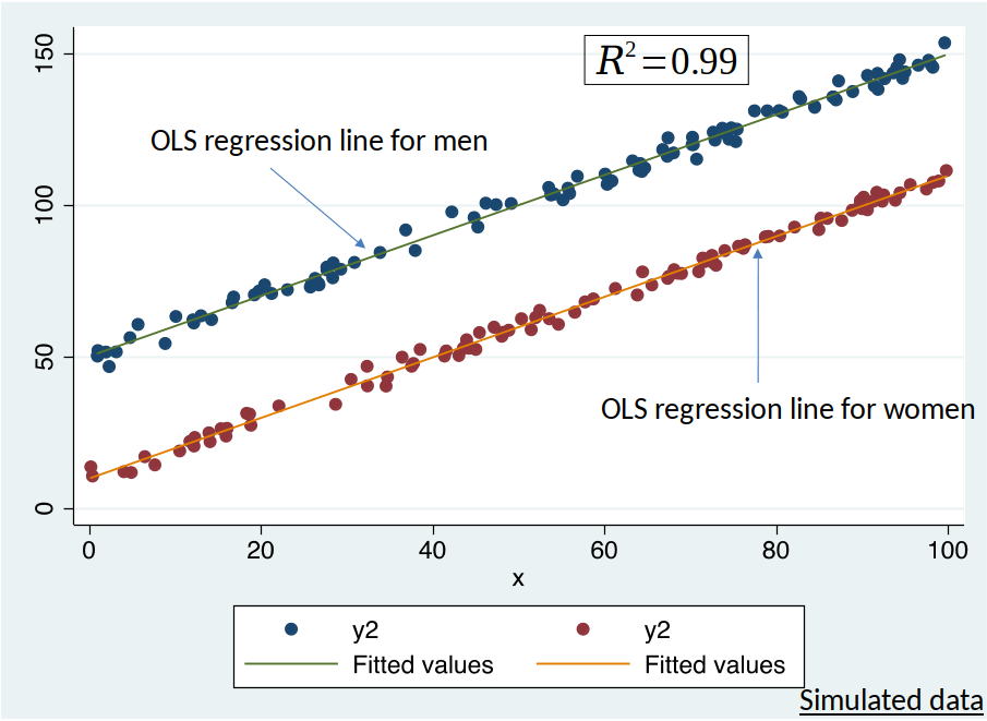
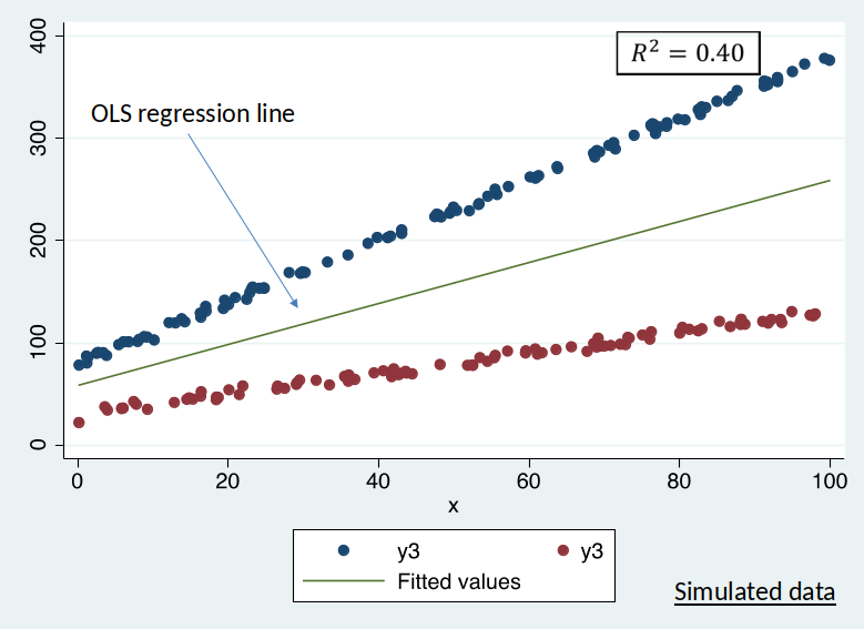
Is OLS regression line a good description of the data?
Seperate DGPs
- When $female=1$ (women): $$ wage = \alpha_0 + \alpha_1 educ + u$$
- When $female=0$ (men): $$ wage = \beta_0 + \beta_1 educ + u$$
- Females and males might have different intercepts ($\alpha_0$ vs $\alpha_1$) and different slopes ($\alpha_1$ vs $\beta_1$).
- Different slopes means that the effect of an increase in education has different effects on wages for women compared to men.
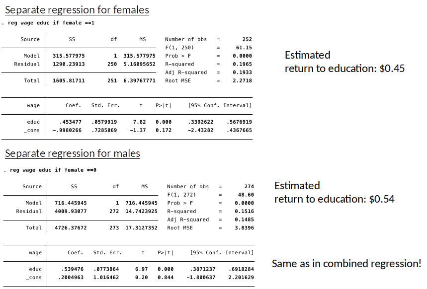
- We can then estimate seperate regression. Or we can combine the two DGPs with the help of an interaction term.
Interaction Term
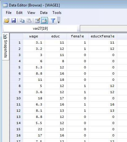
To create an interaction term simply multiply the two variables.
$educXfemale=educ*female$
Combining the DGPs
- Combined DGP, $$ wage = \beta_0 + \delta_0 female + \beta_1 educ + \delta_1 educXfemale + u$$
- DGP for men ($female=0$): $$ wage = \beta_0 + \beta_1 educ + u$$
- DGP for women ($female=1$):
$$ wage = \beta_0 + \delta_0 + \beta_1 educ + \delta_1 educ + u$$
- Intercept for females: $\beta_0+\delta_0$
- Slope (return to education) for females: $\beta_1+\delta_1$
Let's estimate the following model: $ wage = \beta_0 + \delta_0 female + \beta_1 educ + \delta_1 educXfemale + u$
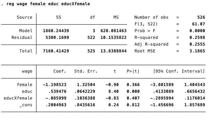
- Estimated return to education for men: 0.54
Estimated return to education for women: 0.54 – 0.09 = 0.45
Is the estimated return to education significantly different for men compared to women?
No, because the p-value on the interaction term educXfemale is 0.407
Advantage of estimating this in one regression is that we can immediately see if the difference is statistically significant.
White referees call more fouls on black players?

Or white referees call less fouls on white players?
We often observe differences in outcomes, but...
Problem 1: These differences could be due to differences in “skill” or actual behaviour?
Even if people would have the same “skills” (i.e. everything else is the same)…
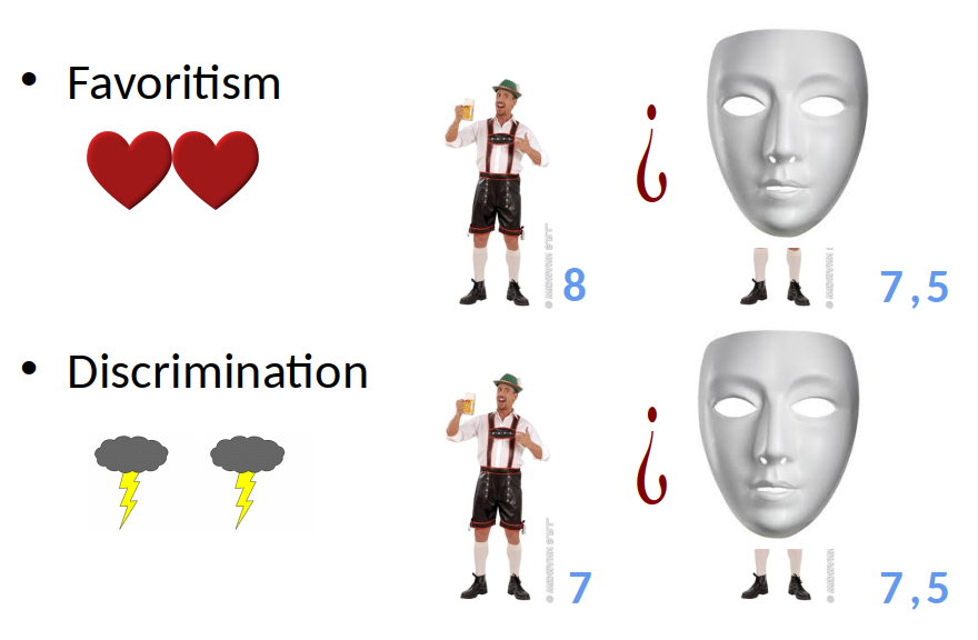
Problem 2: These differences could be due to discrimination or favouritism?
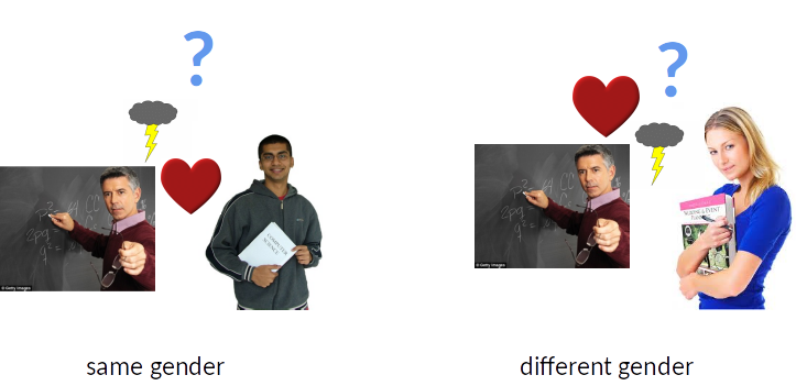
Example: Discrimination in Exam Grading
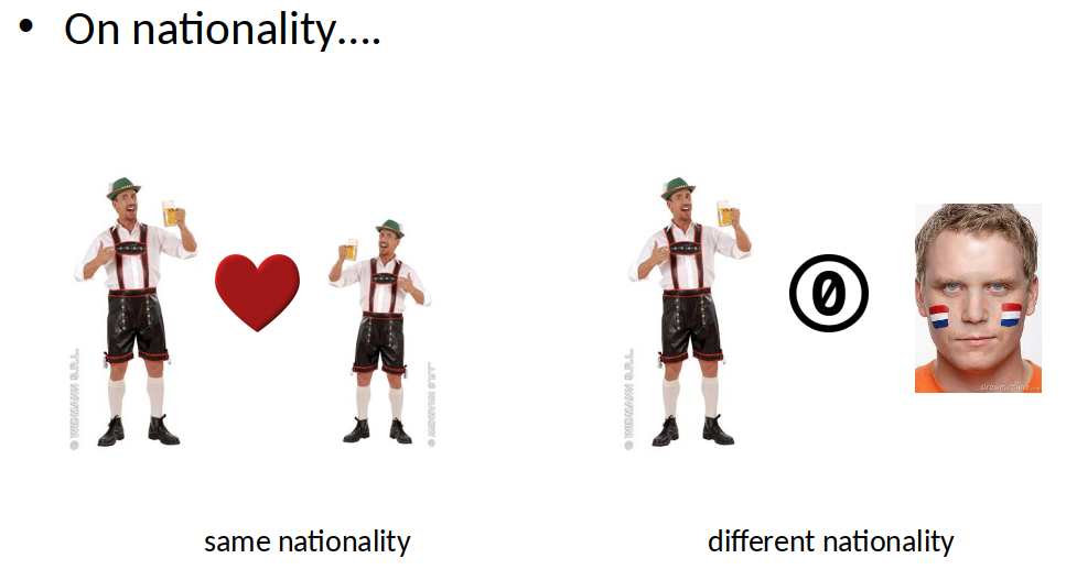
- How do graders grade students with the same/different nationality?
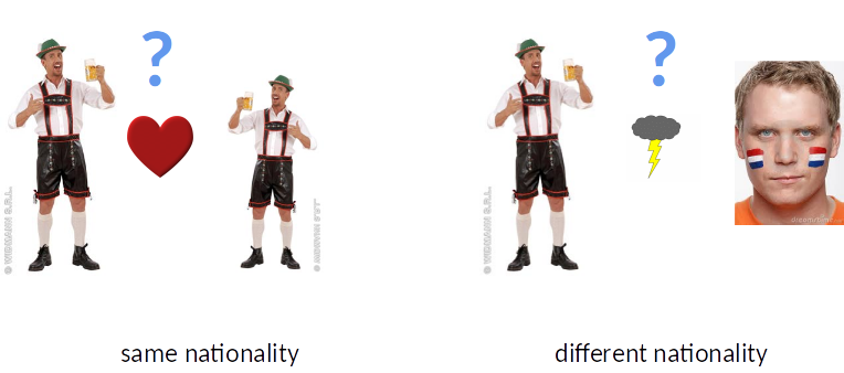
- How do graders grade students with the same/different gender?

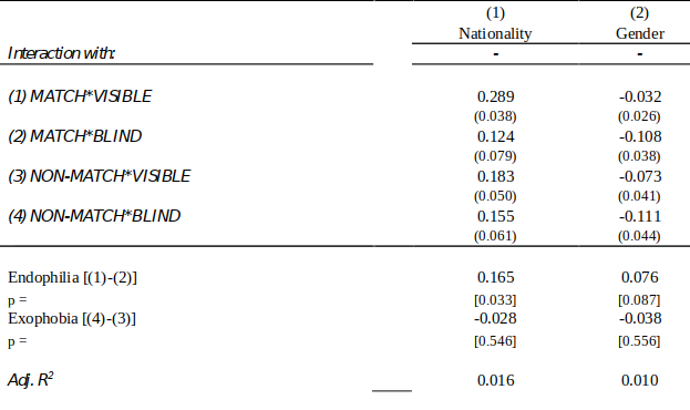
Empirical Strategy
$$ S = \beta_1 MATCH*VISIBLE + \beta_2 MATCH*BLIND + \beta_3 NON-MATCH*VISIBLE + \beta_4 NON-MATCH*BLIND + \gamma’ Z + \epsilon $$
S = Exam score per question (standardised)
Z = student and grader gender and nationality.
Endophilia = S|VISIBLE,MATCH – S|BLIND,MATCH $= \beta_1 – \beta_2$
Exophobia = -1*[S|VISIBLE,NON-MATCH – S|BLIND,NON-MATCH] $= \beta_4 – \beta_3$
Results
- Do you want to guess the results?
- Do you want to guess the results?
What should you take home?
- Next time you hear about “discrimination”… recall that:
- this might be due to differences in “skill” (i.e. everything else)
- And it might be also be favoritism

See paper: Jan Feld, Nicolas Salamanca and Daniel S. Hamermesh, (2016) “Endophilia or Exophobia: Beyond Discrimination”, The Economic Journal