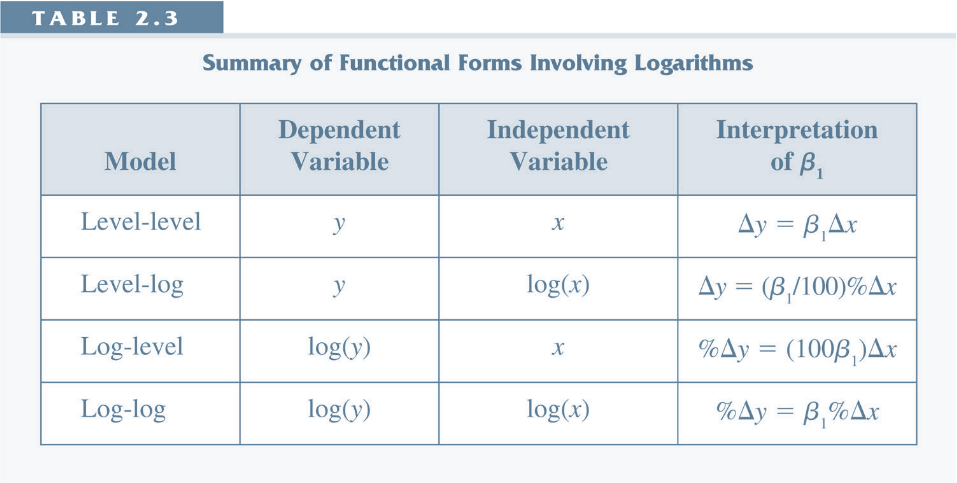
Further Issues
- Quadratic relationships
- Exponential relationships
- Consistency
- Adjusted R-squared
- Data scaling
Reference: Wooldridge, Chapters 5-6
Linearity Assumption
This model implies that the effect of x on y is linear (i.e., the same for all levels of x).
$y=\beta_0 + \beta_1 x + u$ Do all DGPs follow this form?
Will an estimate of a linear effect always be the best description of the data?
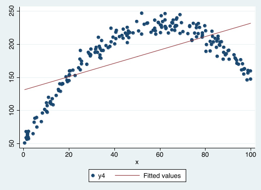
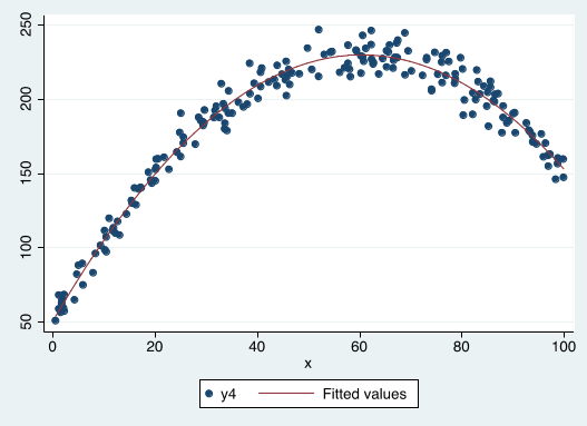
Can we estimate a simple linear regression in this case?
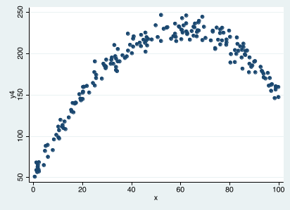
Is the OLS regression line a good description of the data?
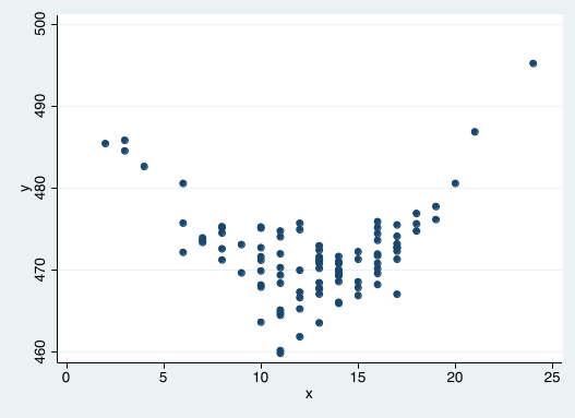
Expressing quadratic DGPs by adding a square term
$$y=\beta_0+\beta_1 x +\beta_2 x^2+u$$
- This way we can express u-shaped and inverse-u-shaped relationships.
For positive values of $x$:
- If $\beta_1>0$ and $\beta_2<0$
- If $\beta_1<0$ and $\beta_2>0$
Marginal effect quadratic relationships in the DGP
$$y=\beta_0+\beta_1 x +\beta_2 x^2+u$$
- Note that $\beta_1$ and $\beta_2$ always have to be interpreted $together$. We get the marginal effect of $x$ on $y$ by taking the first derivative with respect to $x$, $$ \frac{\Delta y}{\Delta x} \simeq \beta_1+2\beta_2 x$$
- The maximum/minimum is at the point $$ x= | \beta_1 / (2\beta_2) | $$
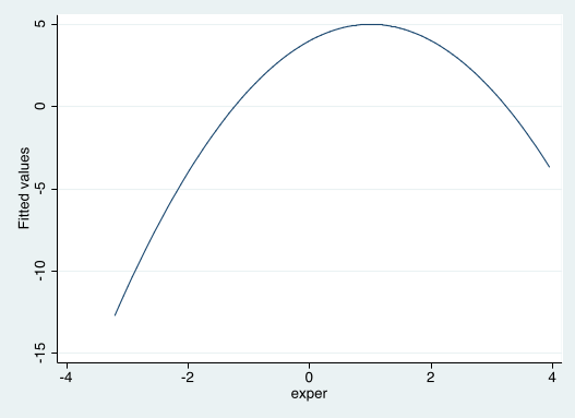
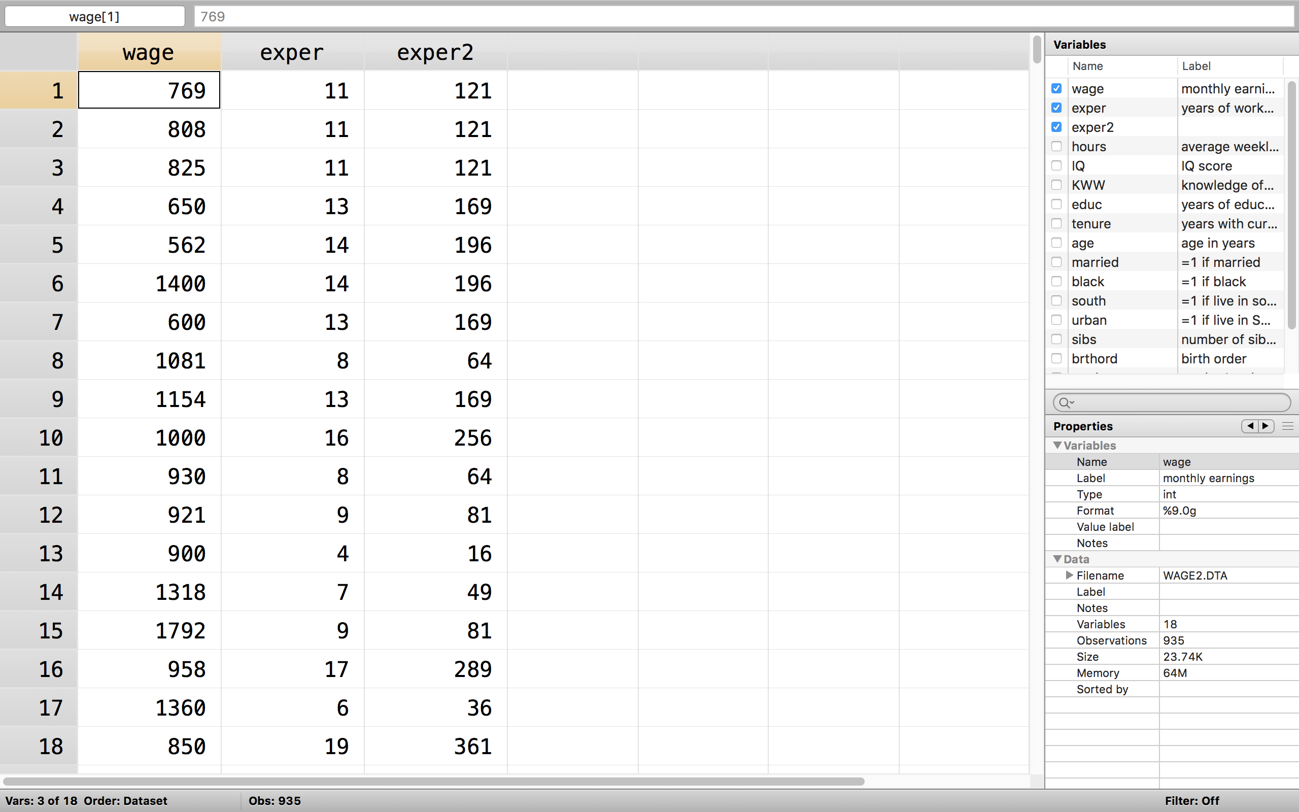
Let's estimate the following model: $$wage= \beta_0+\beta_1 exper +\beta_2 exper^2+u$$
Step 1: Generate the squared term ($exper^2$). [Stata: gen exper2=exper*exper]
Step 2: Include the original variable and the square term in the regression
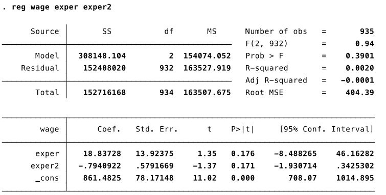
The estimated effect of experience first increases, and then decreases with experience.
Note: Because the coefficient exper2 is not significant (p-value 0.171) we can’t reject the null hypothesis that the effect of experience is linear.
However, we know from other datasets that the effect of experience on wage is inverse u-shaped.
To get at the marginal effect of experience on predicted wage, we take the first derivative.
$$ \frac{\Delta \widehat{wage}}{\Delta exper} = \hat{\beta}_1+2\hat{\beta}_2 exper = 18.84-2*0.79*exper $$
The estimated effect of going from 0 to 1 year of experience is equal to approximately $\$18.84$.
The *estimated* effect of going from 20 to 21 years of experience is equal to approximately $-\$12.76$.
The estimated effect of experience is $\$0$ at $\frac{18.84}{1.58}=11.73$ years.
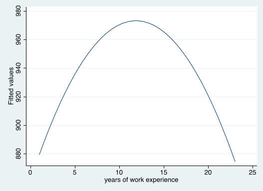
The maximum/minimum is at the point $|\frac{\beta_1}{2\beta_2}|$
Recall MLR.1
Assumption MLR.1: The model is linear in parameters: $y=\beta_0+\beta_1 x_1+\beta_2 x_2 +...+\beta_k x_k + u$
This means we can estimate any model with OLS --even nonlinear relationships-- as long as we can express it with linear parameters (i.e. betas that linearly affect variables).
Example of relationship that is not linear in parameters: $$ f(x,\beta) = \frac{\beta_1 x}{\beta_2 + x}$$
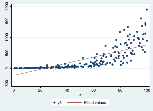
Is this a quadratic relationship?
Can we estimate a simple linear regression with this data?

Is this OLS regression line a good description of the data?
Recap: (compound) interest.
growth = (1+return)$^x$
- Let's say the interest rate is 100%, which is paid once a year.
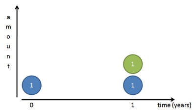
growth = (1+100/100)$^x$=2
Compound interest.
- (Annual) Interest rate 100%. Now you get paid on your interest every 6 months.
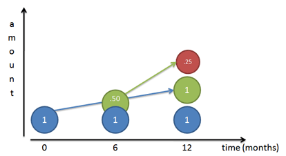
growth = (1+50/100)$^2$=2.25
[50=half of 100, as 6 months is half of one year]
Compound interest.
- (Annual) Interest rate 100%. Now you get paid on your interest every 4 months.
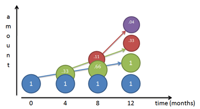
growth = (1+33.3/100)$^3$=2.237037...
[33.3=one third of 100, as 4 months is one third of one year]
Compound interest.
If the rate=1 (ie. 100%) and interest period is indefinitely small, the growth rate is equal to 2.71829...$\equiv e$. $$ \text{Amount(t)=Initial amount} * e^{rate*time} $$
In words: e is the rate of growth if we continuously compont 100% return. $$ growth= e=\lim_{n \to \infty} \left(1+\frac{1}{n} \right)^n$$
Generalization
We can generalize the continuous growth process to other rates. $$ y_t=y_0 * e^{rate*time} $$
Changes in the amount (expressed as a ratio) $$ \text{growth of y} = e^{rate*time} $$
Some changes are not with respect to time, but other variables. We can therefore generalize: $$ \text{growth of y} = e^{rate*x} $$
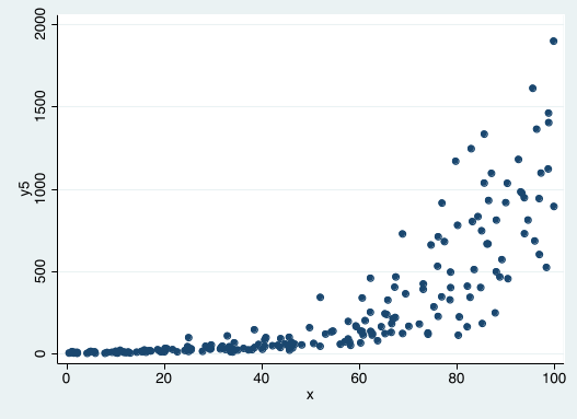
Exponential Relationships
Some DGPs can be characterized by a continuous growth process. In this kind of process the increase depends on the level of y.
Examples
- Interest
- GDP
- Human populations
- Bacteria populations

Exponential GDP
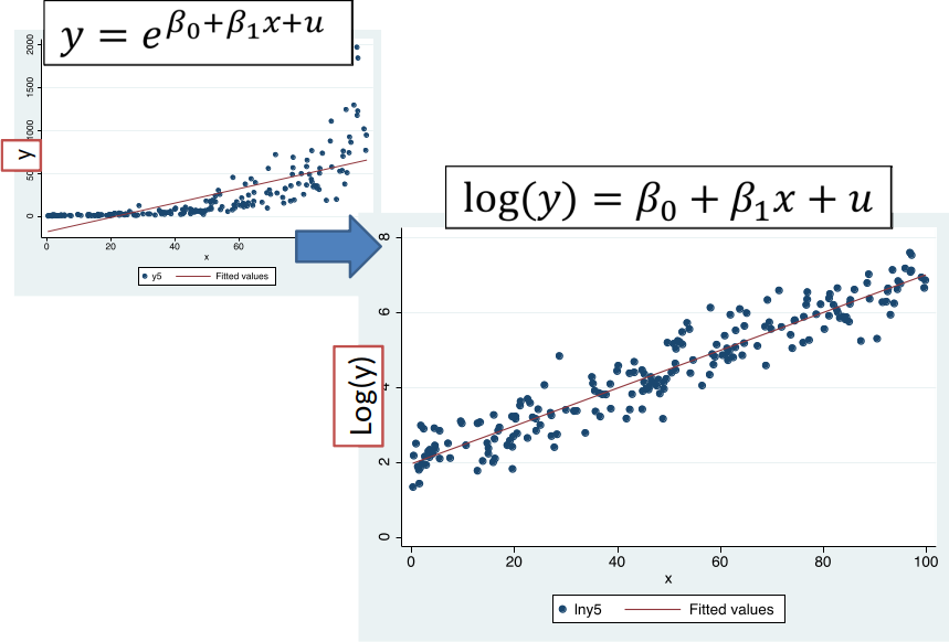
A DGP that is characterized by a continuous growth process can be expressed like this: $$ y= e^{\beta_0 + \beta_1 x + u} $$
This is currently non-linear in parameters. But...
Transform variables...
..to express as a DGP that is linear in parameters (see MLR.1).
If the DGP has the functional form $$ y= e^{\beta_0 + \beta_1 x + u} $$
We can take (natural) log of both sides to get $$ ln(y)=\beta_0 + \beta_1 x + u $$
Marginal Effect
- DGP $y=e^{\beta_0+\beta_1+u}$
- If $\beta_1=1$, if $x$ increases by 1, $y$ increases by a factor of $e^{\beta_1*1}=e^1=2.718$.
- If $\beta_1=0.08$, if $x$ increases by 1, $y$ increases by a factor of $e^{\beta_1*1}=e^{0.08}=1.083$ (approx. 8%).
- Rule of thumb for the above DGP: for small changes, $\beta_j$ is a good approximation of the percentage changes in $y$.
Return to Education
If a one-year increase in education increases the wage by a constant dollar amount, then the DGP would look like $$ y= \beta_0 + \beta_1 x + u $$
If a one-year increase in education increases the wage by a constant percentage, then the DGP would look like $$ y= e^{\beta_0 + \beta_1 x + u} $$
Let's estimate the following model: $wage=\beta_0 + \beta_1 educ + u$
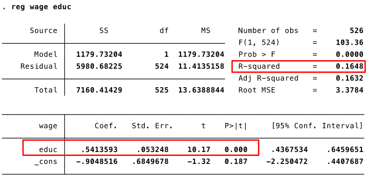
A one-year increase in education increases predicted hourly wage by $\$0.54$.
[Note: deliberately estimating what we suspect is a 'wrong/misspecified' model.]
Let's estimate the following model: $log(wage)=\beta_0 + \beta_1 educ + u$
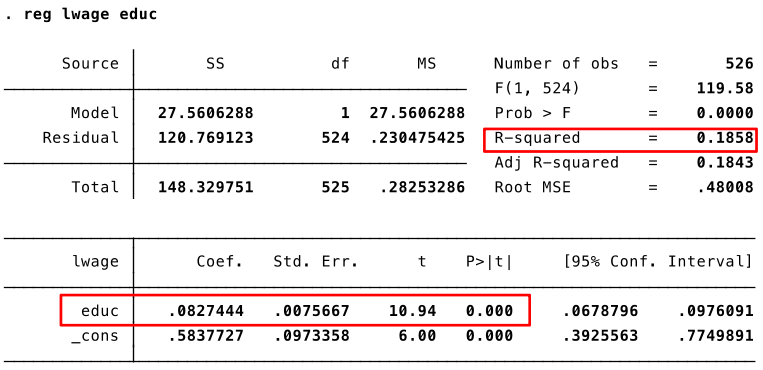
A one-year increase in education increases predicted hourly wage by approximately $8.3\%$.
Comparing the R-squared of the two regressions we can see that the log(wage) model fits the data better.
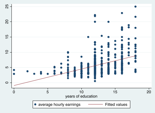
Wage and Education
Interpretation of log-level models
Rule of thumb: for small values of $\beta_j$, $\beta_j$ is a good approximation of percentage changes in y.
This percentage approximation is only good for small values of $\beta_j$.
Calculating the exact percentage difference from a log difference
- General Estimated model: $ log(y)= \beta_0 + \beta_1 x_1 + \beta_2 x_2 + u $
- You can calculate the exact percentage change in $y$ in response to change $\Delta x_j$ using the formula: $$ 100*(e^{\beta_j \Delta x_j}-1) $$
- Note: the exact percentage effect of increasing and decreasing $x_j$ are not the same.
Recall the following regression: $log(wage)=\beta_0 + \beta_1 educ + u$
- A one-year increase in education increases predicted hourly wage by $100*(e^{0.083*1}-1)=8.7$. So, 8.7%.
- A one-year decrease in education increases predicted hourly wage by $100*(e^{0.083*(-1)}-1)=-8$. So, -8%.
- A ten-year increase in education increases predicted hourly wage by $100*(e^{0.083*10}-1)=129$. So, 129%.
Interpretation of log-models
Further points on log models
- They often lead to less heteroskedasticity.
- Estimates are less sensitive to large outliers.
- Rule of thumb: logs are often used when a variable is a positive dollar (or any other currency) amount.
- We cannot take the log of a negative number, or of zeros.
- If y is sometimes zero but never negative, we sometimes use $log(1+y)$.
How to decide on the functional form
- Our starting point is usually to assume that the relationship is linear. But this is not always the case. When deciding on the functional form of your model you can:
- think about the DGP.
- get insight from theory or other empirical evidence (e.g., the effect of age and experience is typically quadratic)
- visually inspect the data (e.g., with scatterplots)
- try different functional forms and compare the R-squared.
- Formally test for functional form misspecification (e.g. regression specification error test, RESET, textbook Chapter 9; not covered in this course).
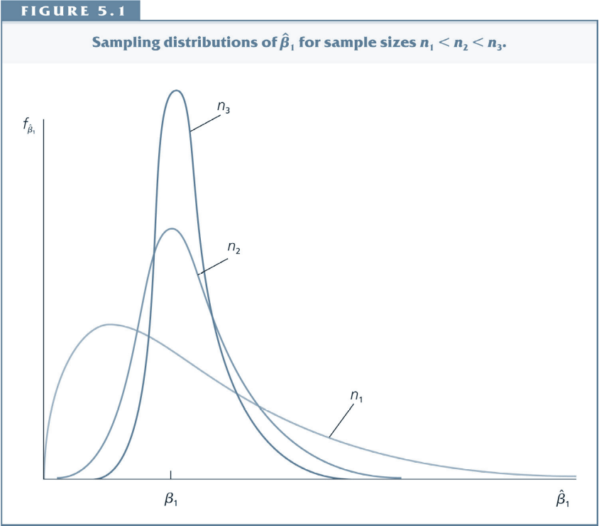
Consistency
Chapter 5 introduces the concept of consistency:
- The estimator becomes more and more tightly distributed around the underlying parameter as the sample grows.
As $n$ (the sample size) tends to infinity, the distribution of $\hat{\beta}_j$ collapses to the single point $\beta_j$.
- This means that we can make our estimator arbitrarily close to $\beta_j$ if we can collect as much data as we want.
- Under assumptions MLR.1-4, $\hat{\beta_j}$ is a consistent estimator of $\beta_j$.
Review (1/2)
What is the functional form of the relationship between x and y?
Write down an econometric model that describes this relationship?
How would you estimate it?
Review (2/2)
What is the functional form of the relationship between x and y?
Write down an econometric model that describes this relationship?
How would you estimate it?
Consistency of $\hat{\beta}_j$
- Good news as n gets very large! The assumptions needed for consistency are less strict than the assumptions needed for unbiasedness.
MLR.4': $E(u)=0$ and $Cov(x_j,u)=0$, for $j=1,2,...,k$
- Under MLR.1-3 and MLR.4': $\hat{\beta}_j$ is a consistent estimator of $\beta_j$.
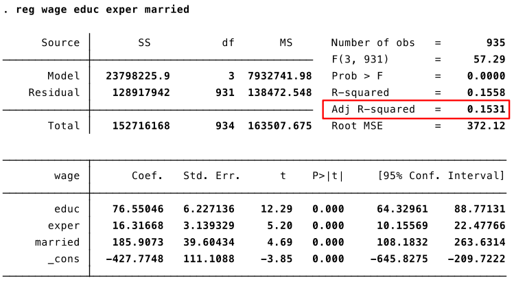
Adjusted R-squared
- We have seen that Stata reports a number called "adjusted R-squared".
- This is an alternative measure of the goodness-of-fit which penalizes the inclusion of additional variables.
- The adjusted R-squared can decrease as you add more explanatory variables.
Comparing (Traditional) R-squared and Adjusted R-squared
(Traditional) R-squared: $R^2 = 1-\frac{SSR/n}{SST/n}$
Adjusted R-squared: $\bar{R}^2 = 1-\frac{SSR/(n-{\color{red}k}-1)}{SST/n-1}$
- Adjusted R-squared penalizes inclusion of more variables (since $k$ increases).
- Adjusted R-squared can even become negative - a very poor model fit!
- Adding an irrelevant variable $x$ (whose coefficient is zero) reduces the adjusted R-squared.
- Adjusted R-squared is occasionally used to choose between models.
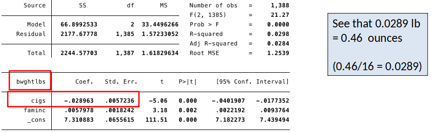
Effects of Data Scaling
(e.g., what if we use 100x instead of x; measure x in cents instead of dollars)
- Everything we expect to happen, does happen.
- Coefficients, standard errors, and confidence intervals change in way that preserves their meanings.
- t-statistics, F-statistics, p-values and $R^2$ remain unchanged.
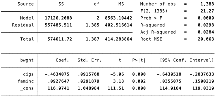
Data Scaling, an example
We are interested in the effects of smoking during pregnancy ($cigs$) and family income ($faminc$) on birthweight ($bwght$): $$\widehat{bwght} = \hat{\beta}_0 + \hat{\beta}_1 cigs + \hat{\beta}_2 faminc$$
$bwght$ is measured in ounces.
- $cigs$ is cigarettes per day during pregnancy.
- $faminc$ is measured in thousands of dollars.
We are interested in the effects of smoking during pregnancy ($cigs$) and family income ($faminc$) on birthweight ($bwght$):
$bwght$ is measured in ounces.
- $cigs$ is cigarettes per day during pregnancy.
- $faminc$ is measured in thousands of dollars.
Interpret the estimated coefficients.
We are interested in the effects of smoking during pregnancy ($cigs$) and family income ($faminc$) on birthweight ($bwght$):
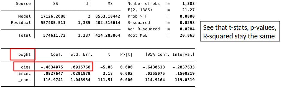
Let’s change $bwght$ from ounces to pounds (1 pound = 16 ounces)
We are interested in the effects of smoking during pregnancy ($cigs$) and family income ($faminc$) on birthweight ($bwght$):
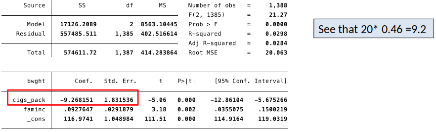
Let’s change $cigs$ from to packs of cigarettes (1 ppack = 20 cigarettes)
Review/Other
Most Important Formulas I
Slope coefficient of Simple Regression Model: $$ \hat{\beta}_1= \frac{Cov(x,y)}{Var(x)} $$
Constant of a Simple Regression Model: $$ \hat{\beta}_0= \bar{y}-\hat{\beta}_1 \bar{x} $$
Most Important Formulas II
Variance of the OLS estimator:
Simple regression model: $$ Var(\hat{\beta}_1)= \frac{\sigma^2}{\sum_{i=1}^n (x_i-\bar{x})^2} $$
Multiple Regression Model: $$ Var(\hat{\beta}_j)= \frac{\sigma^2}{SST_j (1-R^2_j)} $$
Most Important Formulas III
Standard Errors of the OLS estimator: $$ se(\hat{\beta}_j)= \frac{\hat{\sigma}^2}{\sqrt{SST_j (1-R^2_j})} $$
t-statistic/t-ratio:
- The standard case, $H0: \beta_j=0$ $$ t_{\hat{\beta}_j}= \frac{\hat{\beta}_j}{se(\hat{\beta}_j)}$$
- The case, $H0: \beta_j=a_j$ $$ t_{\hat{\beta}_j}= \frac{\hat{\beta}_j-a_j}{se(\hat{\beta}_j)}$$
Most Important Formulas IV
- R-squared $$ R^2 \equiv \frac{SSE}{SST} = 1-\frac{SSR}{SST}$$
- Total Sum of Squares, SST $$ SST \equiv \sum_{i=1}^n (y_i-\bar{y})^2$$
- Explained Sum of Squares, SSE $$ SSE \equiv \sum_{i=1}^n (\hat{y}_i-\bar{y})^2$$
- Residual Sum of Squares, SSR $$ SSR \equiv \sum_{i=1}^n \hat{u}_i^2 = \sum_{i=1}^n (y_i-\hat{y}_i)^2$$ Recall, $SST=SSE+SSR$.