QUAN201 - Introduction to Econometrics

Topic 4: Inference

2020

Intro to Econometrics: Inference

• Normality assumption
• Hypothesis testing: t-test
• Hypothesis testing: F-test

Reference: Wooldridge "Introductory Econometrics - A Modern Approach", Chapter 4

Inference: basic idea

• We can measure $\hat{\beta}$ from our sample, e.g., by using OLS regression.
• We are realy interested in $\beta$.
• Say we get $\hat{\beta}=5$; we know $\hat{\beta}$ has a distribution (different samples would give different values).
• Can we rule out possibility that $\beta=6$? Can we rule out possibility that $\beta=60$?
• What can we confidently infer about $\beta$ based on what we find for $\hat{\beta}$ in our sample?
• More generally: What can we infer about the population, based on our sample?

What does our OLS estimator tell us about the DGP?

• Recall the “I love numbers”-course experiments of not-my brother?

  

• The first OLS estimate suggested that each course increases the math score by 0.15 points ($\hat{\beta}_1=0.15$)…

  

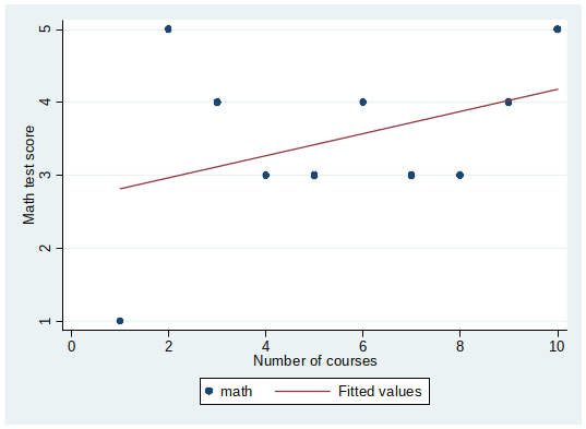
• But that was only one estimate….

What does our OLS estimator tell us about the DGP?

• For each new random sample we would usually get a different estimate.

• So what can we learn about the true value of $\beta_j$ from $\hat{\beta}_j$ in one sample? (We usually only have one sample!)

• If MLR 1-4 hold, $\hat{\beta}_j$ is our best guess for the true value of $\beta_j$. But, we want to know:

  • Is the effect “real” or a result of chance?
  • How close can we expect $\beta_j$ to be to $\hat{\beta}_j$?

Hypothesis testing, intuition

• How would you decide if an estimate is evidence of a ”real” effect (i.e. the true effect is not zero) and not a result of chance?

• Recall that we can estimate the variance of an OLS estimator.

• An estimate is more likely the result of a ”real” effect if:

  • The estimated value is large in absolute terms.
  • The variance of the estimator is small.

Hypothesis testing, outline

• We sometimes want to know whether an effect is ”real” or just a result of chance ($\beta_j = 0$).
  • Null hypothesis (H0): $\beta_j = 0$ (there is no effect, our $\hat{\beta}_j$ is due to chance)
  • Alternative hypothesis (H1): $\beta_j \neq 0$ (the effect is ”real”)

Recap Normal Distribution

$X$ is normally distributed with mean $\mu$ and standard devidation $\sigma$

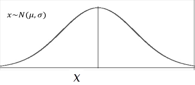
What are the properties of the normal distribution?

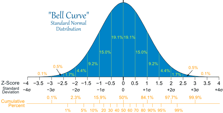
We can standardize a normal distribution by $\frac{x-\mu}{\sigma} \to N(0,1)$

Problem

• Our $\hat{\beta}_j$ is drawn from a distribution.
• The standard error of $\hat{\beta}_j$ tells us how wide this distribution is.
• We don’t know the shape of the distribution of $\hat{\beta}_j$.

Different distributions

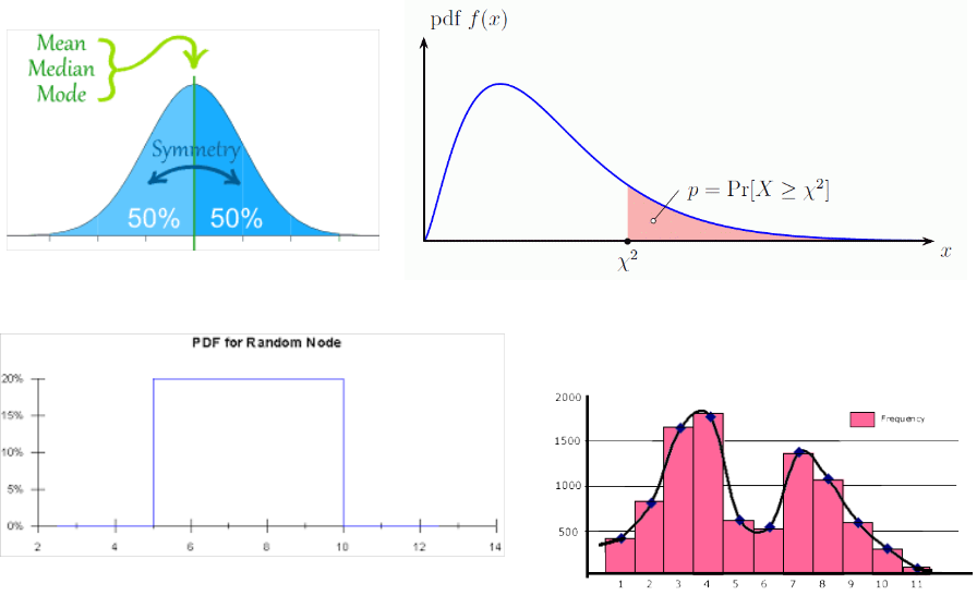
[Advanced technical footnote: any function that is non-negative and integrates (adds up to) 1 is the pdf of a distribution.]

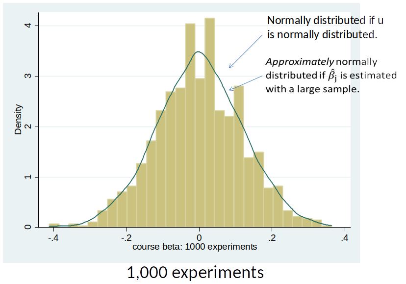
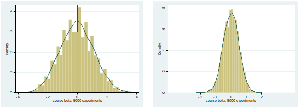
Distribution of $\hat{\beta}_j$

• $\hat{\beta}_j$ is normally distributed if:

  • the error term $u$ is normally distributed

• $\hat{\beta}_j$ is approximately normally distributed if:

  • we have large samples

Empirical Distribution of $\hat{\beta}_j$

Hypothesis testing, short

• The means and standard deviations of $\hat{\beta}_j$ depend on the context.
  • If $\hat{\beta}_j$ is unbiased, the mean is equal to $\beta_j$
  • The standard deviation also depends, among other things, on the sample size (see formula for variance of $\hat{\beta}_j$)

Hypothesis testing, short

• We therefore have to standardize: Under MLR 1-6 one can show that:

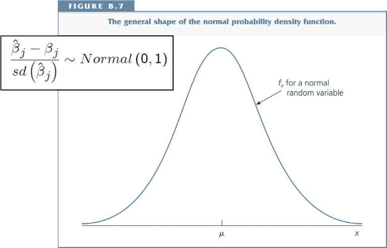
  • The ratio of $\hat{\beta}_j - \beta_j$ to the standard deviation follows a standard normal distribution.

    

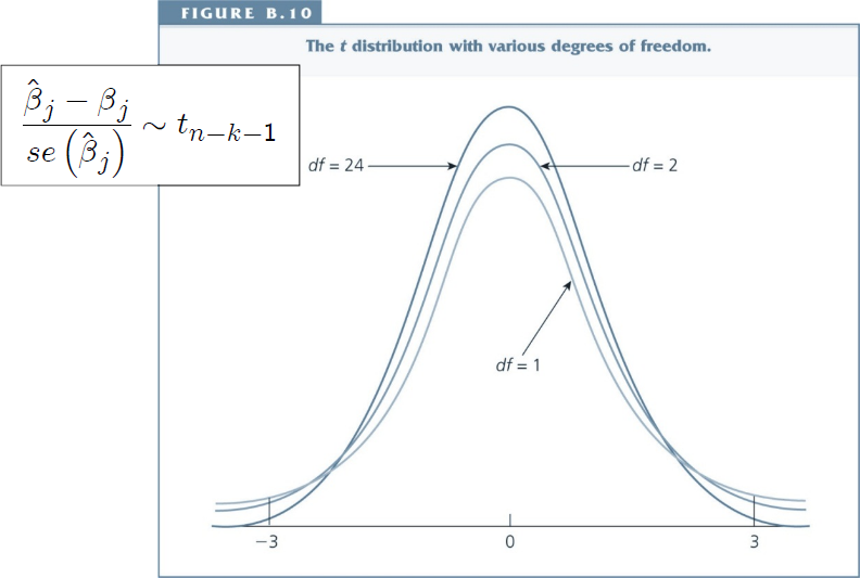
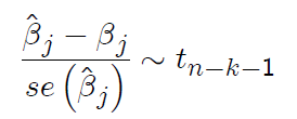
  • The ratio of $\hat{\beta}_j - \beta_j$ to the standard error (called t-statistic) follows a t-distribution.

    

The normal distribution

The t distribution

Hypothesis Testing, short

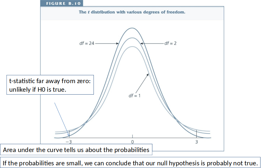
We can then ask: If the hypothesized value of $\beta_j$ is true (usually $\beta_j=0$), what is the probability of observing a t-statistic as extreme as the one we have?

Each value of the t-statistic is associated with a specific probability: If this probability is low, we conclude that the hypothesized value is probably not true.

Hypothesis Testing, short

Review: Hypothesis Testing

Goal: find out whether $\beta_j$ is different from zero?

Remember that $\hat{\beta}_j$ has a distribution?

Empirical Distribution of $\hat{\beta}_j$

We can standardize a normal distribution by $\frac{x-\mu}{\sigma} \to N(0,1)$

Hypothesis Testing, short

• We therefore have to standardize: Under MLR 1-6 one can show that:

  • The ratio of $\hat{\beta}_j - \beta_j$ to the standard deviation follows a standard normal distribution.

    

  • The ratio of $\hat{\beta}_j - \beta_j$ to the standard error (called t-statistic) follows a t-distribution.

    

We assume that null hypothesis is true (typically $\beta_j = 0$)

Calculate t-statistic: $\frac{\hat{\beta}_j-0}{se(\hat{\beta}_j)}$

Hypothesis Testing, short

Hypothesis testing, step by step

We continue to make assumptions MLR.1-5 introduced previously.

We additionally assume that the unobserved error term ($u$) is normally distributed in the population.

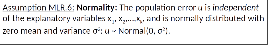
This is often referred to as the normality assumption. (Note that non-normality of $u$ is not a problem if we have large samples)

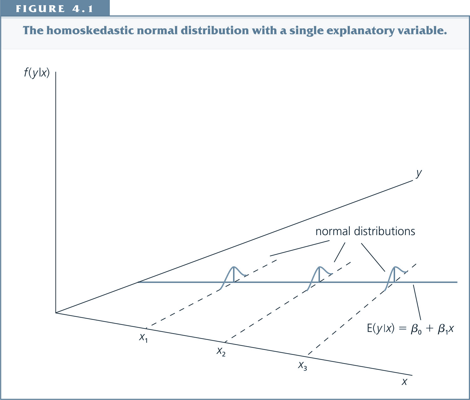
Under the classical linear model (CLM) assumptions (MLR 1. -6.), the error term u is normally distributed with constant variance (the latter due to homoskedasticity):

But why are we assuming normality?

Answer: It implies that the OLS estimator $\hat{\beta}_j$ follows a normal distribution too.
Theorem 4.1: Under the CLM assumptions (MLR.1-6): $$\hat{\beta}_j \sim Normal(\beta_j,Var(\hat{\beta}_j))$$

where $$ Var(\hat{\beta}_j) = \frac{\sigma^2}{SST_j (1-R^2_j)} $$

[Do you remember how the R-squared is defined? Why does it have a j-subscript? If you’re not sure, check the the slides for topic 3.]

The result that $\hat{\beta}_j \sim Normal(\beta_j, Var(\hat{\beta}_j))$
implies that

where $$ sd(\hat{\beta}_j)= \sqrt{Var(\hat{\beta}_j)}=\frac{\sigma}{\sqrt{SST_j (1-R_j^2)}} $$

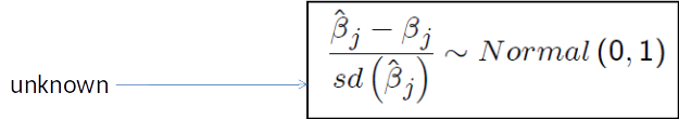
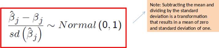
In words: the difference between the estimated value and the true parameter value, divided by the standard deviation of the estimator, is normally distributed with mean 0 and standard deviation equal to 1.

$$\frac{\hat{\beta}_j - \beta_j}{sd(\hat{\beta}_j)} \sim Normal(0, 1)$$

Note, we don’t observe $sd(\hat{\beta}_j)$, because it depends on $\sigma$ (the standard deviation of the error term $u$), which is an unknown parameter.

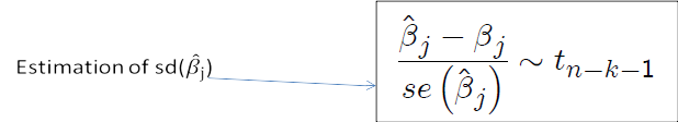
But we can calculated the standard error $se(\hat{\beta}_j)$ which is an estimate of $sd(\hat{\beta}_j)$.

If we replace $sd(\hat{\beta}_j)$ with $se(\hat{\beta}_j)$ we get the t-statistic, which follows a t-distribution instead of a normal distribution.

The test is therefore often referred to as a t-test.

_{^{[Technical footnote: $sd(\hat{\beta}_j)$ is a number. The normal distribution minus a number divided by a number gives us a (different) normal distribution. $se(\hat{\beta}_j)$ in contrast has a distribution (namely it follows a chi-squared distribution) hence why we get something different.]}}</sup>

Standard error of $\hat{\beta}_j$

Formula for standard error: $$ se(\hat{\beta}_j)= \sqrt{Var(\hat{\beta}_j)}=\frac{\hat{\sigma}}{\sqrt{SST_j (1-R_j^2)}} $$

Where $\hat{\sigma}$ is based on the OLS residuals, $$ \hat{\sigma}^2 = \frac{SSR}{n-k-1} = \frac{\sum_{i=1}^n (\hat{u}_i)^2 }{n-k-1} $$

t-statistic

The t statistic or the t ratio of $\hat{\beta}_j$ is defined as:

The standard case (If $H_0: \beta_j=0$): $t_{\hat{\beta}_j} = \frac{\hat{\beta}_j}{se(\hat{\beta}_j)}$

[General case (If $H_0: \beta_j=a_j$): $t = \frac{\hat{\beta}_j-a_j}{se(\hat{\beta}_j)}$ ]

• For the standard case, the t-statistic is easy to compute: just divide your coefficient estimate by the standard error.
• Stata will do this for you.
• Since the se is always positive, the t-statistic always has the same sign as the coefficient estimate.

t-statistics in Stata

Quiz: Calculate the t-statistic for skipped.

t distribution for the Standardized Estimators

under the CLM assumptions:

$$\frac{\hat{\beta}_j - \beta_j}{se(\hat{\beta}_j)} \sim t_{n-k-1}$$

where $k+1$ is the number of unknown parameters in the population model ($k$ slope parameters & the intercept).

In words, this says that the difference between the estimated value and the true parameter value, divided by the standard error of the estimator follows a t-distribution with $n-k-1$ degrees of freedom .

Shape of the t-distribution

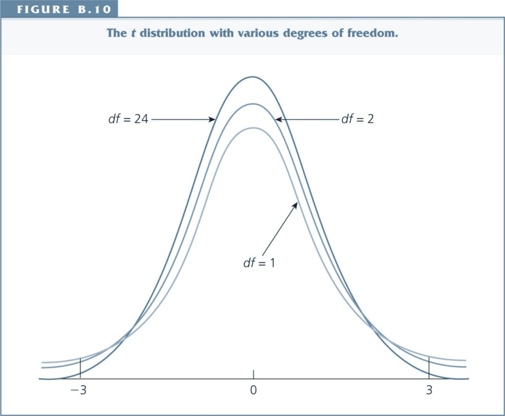
• The shape is similar to the standard normal distribution - but more spread out and more area in the tails.
• As the degrees of freedom increases (e.g. when n increases), the t distribution approaches the standard normal distribution.

Testing hypotheses about a single parameter of the DGP: The t test

Our starting point is the model (DGP): $$ y= \beta_0 + \beta_1 x_1 + \beta_2 x_2 + ... + \beta_k x_k +u $$

Our goal is to test hypotheses about a particular $\beta_j$

Remember: $\beta_j$ is an unknown parameter and we will never know its value with certainty. But we can hypothesize about the value of $\beta_j$ and then use statistical inference to test our hypothesis.

Hypothesis testing, step by step for two sided alternatives (standard case)

Step $1$. Specify null hypothesis (H0) and alternative Hypothesis (H1).
H0: $\beta_j = 0$
H1: $\beta_j \neq 0$ (two sided alternative)

Step $2$. Decide on a significance level ($\alpha$): highest probability we are willing to accept of rejecting H0 if it is in fact true.
The most common significance level is 5%.

Hypothesis testing, step by step

Step $3$. Stata computes the t-statistic and looks up the p-value associated with it.

Example:

Suppose t = 1.85 and df=40.

This results in a p-value = 0.0718.

p-values in Stata

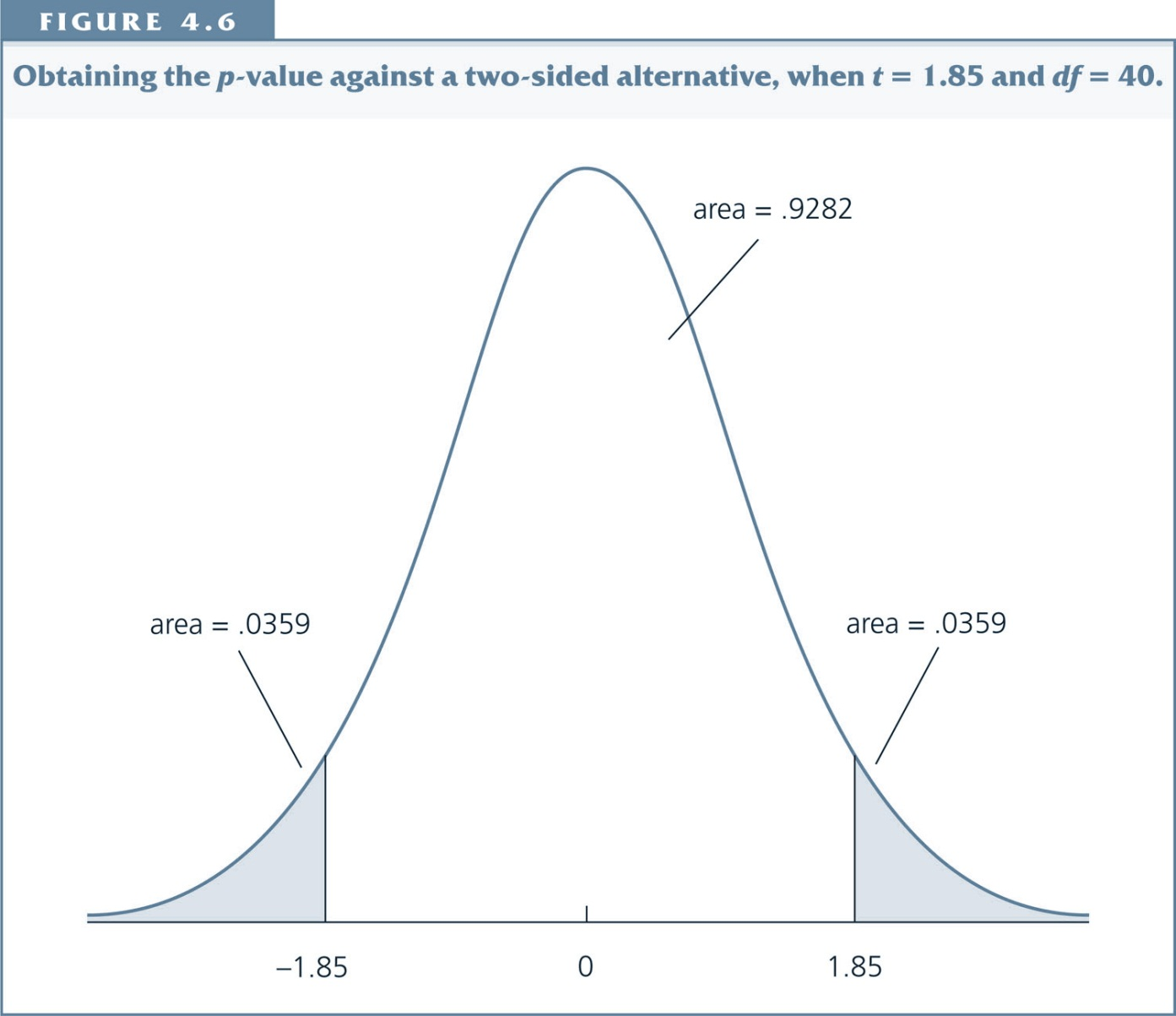
Interpretation: The p-value is the probability of observing a t-statistic as extreme as we did if the null hypothesis is true.

Thus, small p-values are evidence against the null hypothesis.

Hypothesis testing, step by step

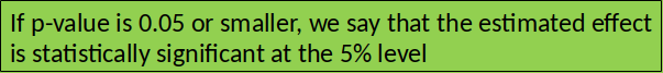
Step $4$. Compare significance level ($\alpha$) with p-value. Decision rule:
If $p-value>\alpha, \quad$ H0 is not rejected.
If $p-value \leq \alpha, \quad$ H0 is rejected in favor of H1.

Rule of thumb

If you can’t look up the p-value, this simple rule of thumb can help:

• For two sided alternatives, 5% significance level and df > 60:
• t-statistic lower than -2 or higher than 2 implies statistical significance. (i.e. We can reject the null hypothesis.)

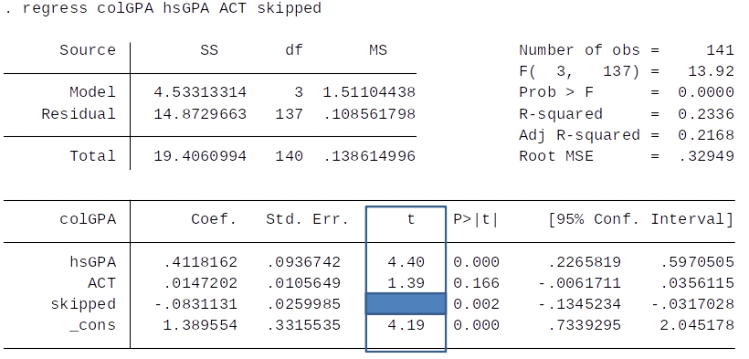
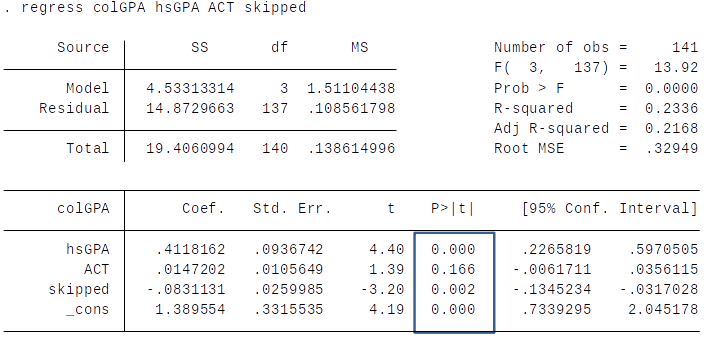
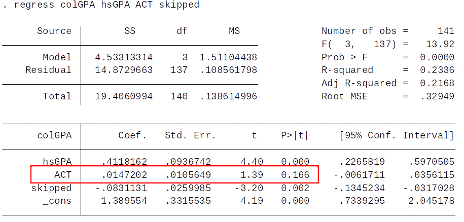
Practice rule of thumb

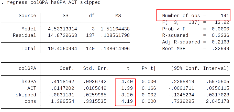
Given our rule of thumb, what can we say about the statistical significance at the 5% level of ACT and skipped?

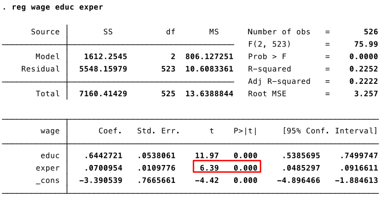
Example: effect of experience on wage

$$ wage = \beta_0 + \beta_1 educ + \beta_2 exper + u $$

The null hypothesis $H0: \beta_2=0$, years of experience has no effect on wage.

H0: $\beta_2=0$
H1: $\beta_2 \neq 0$

Significance level: 5%

Assume that CLM hold.

(continues next slide)

(answer next slide)

t-statistic: 6.39, p-value: 0.000

Significance level > p-value $\to$ reject H0.

Testing other hypotheses about $\beta_j$

Although H0: $\beta_j=0$ is the most common hypothesis, we sometimes want to test whether $\beta_j$ is equal to some other given constant. Suppose the null hypothesis is $$ H0: \, \beta_j=a_j$$

In this case the appropriate t-statistic is: $$t = \frac{\hat{\beta}_j-a_j}{se(\hat{\beta}_j)}$$

The rest of the t-test is the same.

Question for Class

Is the hsGPA coefficient in the regression below significantly different from 1 (against a two-sided alternative) at the 5% level?

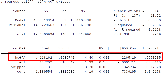
A) Yes B) No C) We can’t say

4.3 Confidence intervals

Once we have estimated the DGP parameters $\beta_0$,$\beta_1$,...,$\beta_k$, and obtained the associated standard errors, we can easily construct a confidence interval (CI) for each $\beta_j$.

The CI provides a range of likely values for the unknown $\beta_j$.

Recall that $\frac{\hat{\beta}_j-\beta_j}{se(\hat{\beta}_j)}$ has a t distribution with $n-k-1$ degrees of freedom (df).

Define a 95% confidence interval for $\beta_j$ as $$ \hat{\beta}_j \pm c \cdot se(\hat{\beta}_j) $$ where constant $c$ the $97.5^{th}$ percentile in the $t_{n-k-1}$ distribution.

_{^{Question: why 97.5, not 95?}}</sup>

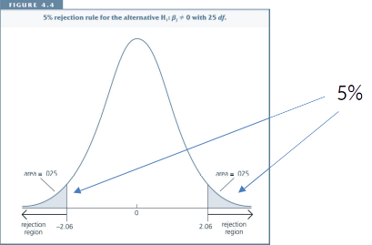
Critical Value

For a 95% Confidence-Interval, the critical value c is chosen to make the area in each tail equal 2.5%, i.e., c is the 97.5th percentile in the t distribution.

The graph shows that, if df=26, then c=2.06.

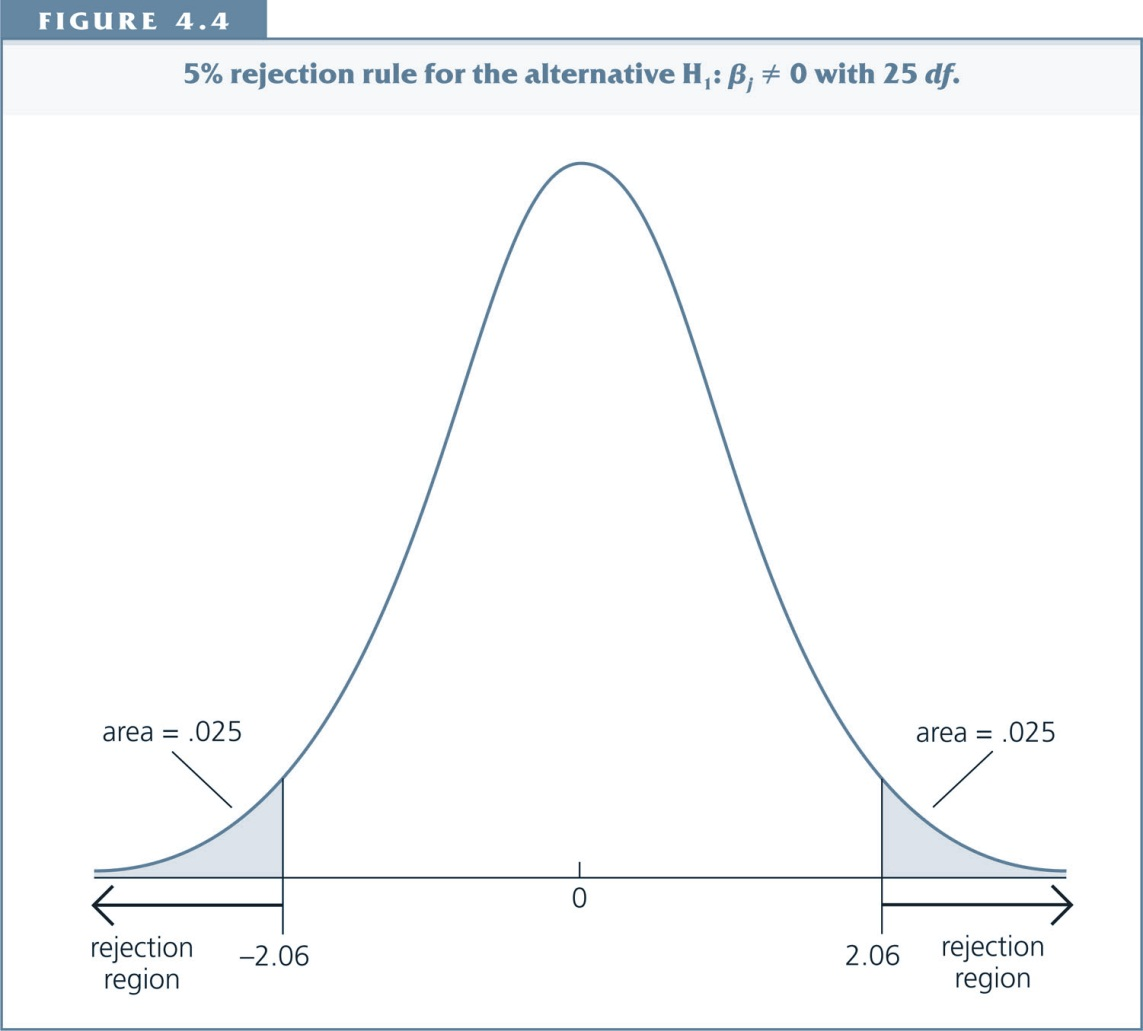
If H0 were true, we would expect a t-statistic larger than 2.06 or smaller than -2.06 in only 5% of the cases.

Confidence intervals (1)

$$ \hat{\beta}_j \pm c \cdot se(\hat{\beta}_j) \left\{ \begin{align*} \bar{\beta}_j = \hat{\beta}_j + c \cdot se(\hat{\beta}_j) \quad \text{upper limit} \\ \underline{\beta}_j = \hat{\beta}_j - c \cdot se(\hat{\beta}_j) \quad \text{lower limit} \end{align*} \right. $$

Constructing a 95% confidence interval involves calculating two values, $\bar{\beta}_j$ and $\underline{\beta}_j$, which are such that if random samples were obtained many times, with the confidence interval ($\bar{\beta}_j$, $\underline{\beta}_j$) computed each time, then 95% of these intervals would contain the unknown.

This implies that if our 95% confidence interval does not include zero, we can reject H0 at the 5% level.

Confidence intervals (2)

$$ \hat{\beta}_j \pm c \cdot se(\hat{\beta}_j) \left\{ \begin{align*} \bar{\beta}_j = \hat{\beta}_j + c \cdot se(\hat{\beta}_j) \quad \text{upper limit} \\ \underline{\beta}_j = \hat{\beta}_j - c \cdot se(\hat{\beta}_j) \quad \text{lower limit} \end{align*} \right. $$

Unfortunately, for the single sample that we use to construct the CI (confidence interval), we do not know whether $\beta_j$ is actually contained in the interval.

We believe we have obtained a sample that is one of the 95% of all samples where the CI contains $\beta_j$, but we have no guarantee.

Question: What happens to the CI when se() increases?

Confidence Intervals in Stata

Assume that CLM assumptions hold.

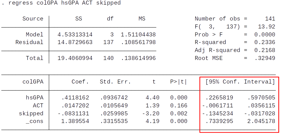
Question: Which coefficient are statistically significant at the 5% level?
Use the Use the 95% CI in your to answer this question.

Do baseball players get paid according to their performance?

• What do you think?

• How is it in other sports?

  

• Let’s find out! We have data on salary and performance statistics.

[Personal thoughts: Baseball is a contender for the worst sport ever invented. This is clear from the fact that the most exciting thing in the game is when the ball is no longer on the field. :P]

Baseball, Model and Data

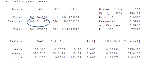
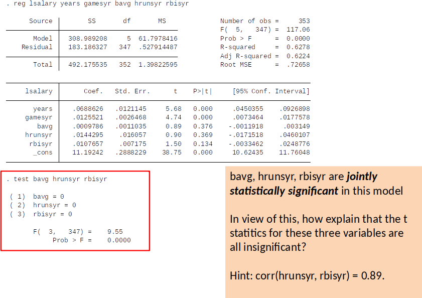
Consider the following model of (major league) baseball players’ salaries: $$ log(salary) = \beta_0 + \beta_1 years + \beta_2 gamesyr + \beta_3 bavg + \beta_4 hrunsyr + \beta_5 rbisyr + u$$

Variables:

• $salary$ = total 1993 salary;
• $years$ = years in the league;
• $gamesyr$ = average games played per year;
• $\color{red}{bavg}$ = career batting average;
• $\color{red}{hrunsyr}$ = home runs per year;
• $\color{red}{rbisyr}$ = runs batted per year

[We will consider the last three variables in red as those capturing 'performance'.]

OLS estimates

Assume that CLM assumptions hold.

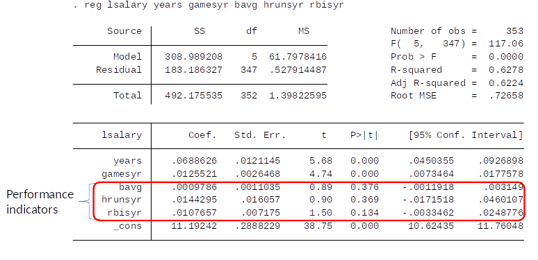
• So each of the coefficients is statistically insignificiant.
• Does that imply we should not reject H0?

Note: Because the dependent variable is log salary, we interpret the coefficients as percentage change in salary. For example, the model predicts that a one year increase in the league increases salary by 6.8%.

What is our hypothesis?

$$ log(salary) = \beta_0 + \beta_1 years + \beta_2 gamesyr + \beta_3 bavg + \beta_4 hrunsyr + \beta_5 rbisyr + u$$

Our hypothesis is very general:
$H0: \beta_3=0, \, \beta_4=0, \, \beta_4=0$
$H1:$ H0 is not true

In economics we sometimes want to test whether a number of coefficients are jointly significant. We can do this with an F-test.

F-test, intuition

• Goal: test whether a group of variables has no effect on the dependent variable.
• Remember the discussion of $R^2$ statistic:
  • We can express y in terms of explained and unexplained part: $y_i = \hat{y}_i+u_i$
  • The total variation in y is equal to the sum of explained and unexplained variation: $$ SST=SSE+SSR $$

$ \text{Sum of Squares Total: }SST= \sum_{i=1}^n (y_i-\bar{y})^2 $
$ \text{Sum of Squares Explained: }SSE= \sum_{i=1}^n (\hat{y}_i - \bar{y})^2 $
$ \text{Sum of Squares Residual: }SSR= \sum_{i=1}^n (\hat{u}_i)^2 $

F-test, intuition

• What happens when our model becomes better at explaining the variation in $y$?
  • SSE increases and SSR decreases
• Remember, $R^2$ always increases when we include more variables.
• The F-test tells us if the reduction in SSR from adding a group of variables is large enough that we can reject $H0$.

F-test, step by step

We compare the SSR of the restricted model to the SSR of the unrestricted model.

Unrestricted model: $$ log(salary) = \beta_0 + \beta_1 years + \beta_2 gamesyr + \beta_3 bavg + \beta_4 hrunsyr + \beta_5 rbisyr + u$$

Restricted model: $$ log(salary) = \beta_0 + \beta_1 years + \beta_2 gamesyr + u$$

Exclusion restrictions: $H0: \beta_3=0, \, \beta_4=0, \, \beta_4=0$

Econometrics jargon: ”impose restrictions” = other values (in our case zeros) are assumed for certain parameters than those obtained when the model is estimated freely. The null hypothesis is that these parameters are "jointly" (all) zero.

Question for Class

What can we say about the relationship between SSRr and SSRur?

a) SSRr ≥ SSRur
b) SSRr ≤ SSRur
c) SSRr = SSRur
d) it depends / we can’t say

[SSRr=SSR of restricted model, SSRur=SSR of unrestricted model]

F-test: key question

When we add the variables to the model and move from the restricted to the unrestricted model...

Key question: Does SSR decrease enough for it to be warranted to reject the null hypothesis?

How much should the SSR decrease so that it is likely not a result of chance, i.e., statistically significant?

The F statistic

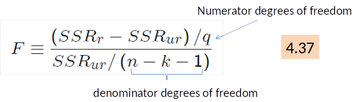
• SSRr is the sum of squared residuals for the restricted model;
• SSRur is the SSR for the unrestricted model.
• $q$ is the number of restrictions imposed in moving from the unrestricted to the restricted model.
• $n-k-1$ = degrees of freedom.
• $n$ is the number of obervations.
• $k$ is the number of variables (in the unrestricted model).

The F statistic & the F distribution

To use the F statistic we must know its sampling distribution under the null (this enables us to choose critical values & rejection rules).

Under $H0$, and when the CLM assumptions hold, F follows an F distribution with (q,n-k-1) degrees of freedom: $$F \sim F_{q,n-k-1}$$

The critical values for significance level of 5% for the F distribution are given in Table G.3.b.

Rejection rule: Reject H0 in favor of H1 at (say) the 5% significance level if F>c, where c is the 95th percentile in the $F_{q,n-k-1}$ distribution.

Unrestricted Model

Restricted Model

$$ F=\frac{(198.311- 183.186)/3}{183.186/347}=9.55 $$

Implication?

Carrying out an F test is easy in Stata…

If we drop $rbisyr$...

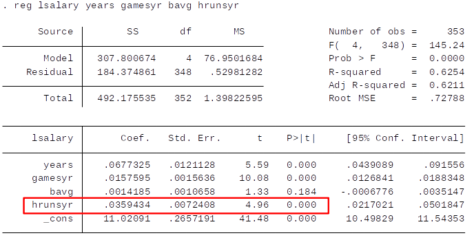
Recall from topic 3: $se(\hat{\beta}_j) = \frac{\hat{\sigma}}{\sqrt{SST_j (1-R_j^2)}}$

This example shows quite clearly that by including near-multicollinear regressors you will get large standard errors and, consequently, low t-values.

Computing p-values for F tests

The p-value is defined as $$ p-value = Pr(\textbf{F}>F)$$

where F is the random variable with $df=(q,n-k-1)$ and $F$ is the actual value of the test statistic.

Interpretation of p-value: The probability of observing a value for F as large as we did given that the null hypothesis is true.

For example, $p-value = 0.016$ implies such probability is only 1.6% - hence we would reject the null hypothesis at the 5% level (but not at the 1% level).

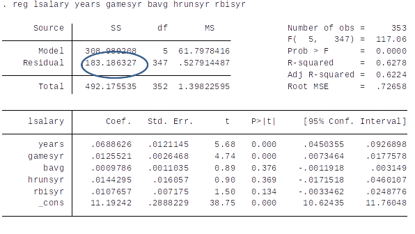
The F statistic for overall significance of a regression

Consider the following model and null hypothesis: $$ y= \beta_0 + \beta_1 x_1 + \beta_2 x_2 + ... + \beta_k x_k +u $$

H0: $x_1, x_2,..., x_k$ do not help to explain $y$
That is,
$H0: \beta_1=\beta_2=...=\beta_k=0$

Model under $H0$: $y=\beta_0 + u$

It can be shown that, in this case, the F statistic can be computed as $$ F=\frac{R^2/k}{(1-R^2)/(n-k-1)}$$

[Note: This last formula is only valid if you want to test whether all explanatory variables are jointly significant. (Thought: If you used the earlier formula, what is $q$ here?)]

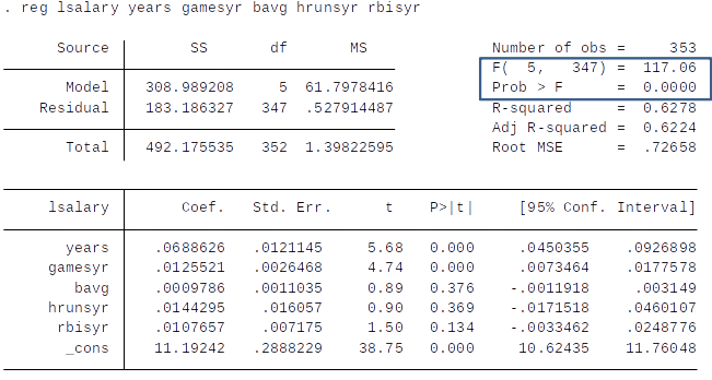
$$ F=\frac{R^2/k}{(1-R^2)/(n-k-1)}=\frac{0.628/5}{(1-0.628)/347}=117$$

• This type of test determines the overall significance of the regression.
• If we fail to reject the null hypothesis, our model has very little explanatory power – it is not a statistically significant improvement over a model with no explanatory variables!
• In such a case, we should probably look for other explanatory variables...

Hypothesis testing, special case: one sided alternative

In some cases, the alternative Hypothesis is only one sided.

H0: $\beta_j=0$
H1: $\beta_j>0$ or H1: $\beta_j<0$

If H1: $\beta_j=0$ this means that we believe that the effect of $x_j$ can only be positive.

Hypothesis testing: one sided alternative

The p-values reported in Stata are for two-sided tests (i.e. H0: $\beta_j=0$, and H1: $\beta_j\neq 0$)

To get the p-value for a one sided test, we just divide the p-value reported in Stata by 2.

Standard Case: Two sided alternative

$$\text{H0: }\beta_j=0\text{, and H1: } \beta_j\neq 0$$

Significance level = 5% $\to$ We accept being wrong in 5% of the cases.
Extreme t-statistics (both positive and negative) are evidence against the null hypothesis.
Choose critical value for which we would be wrong in 5% of the cases.

Special Case: One sided alternative

$$\text{H0: }\beta_j=0\text{, and H1: } \beta_j > 0$$

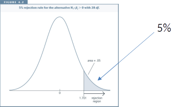
Significance level = 5% $\to$ We accept being wrong in 5% of the cases.
Large, positive t-statistics are evidence against the null hypothesis.
Large, negative t-statistics are evidence for the null hypothesis.
Choose critical value for which we would be wrong in 5% of the cases.

One sided is less conservative

One sided hypothesis testing less conservative:

• Critical values are smaller
• p-values are smaller (1/2 size)

This is because we already rule out one direction of the effect.

Hypothesis testing, one sided alternative

The key difference is that we look up a different critical value.
Step 1: Specify null and alternative hypothesis (H0: $\beta_j=0$; H1: $\beta_j>0$ (or H1:$\beta_j<0$))
Step 2: Decide on significance level.
Step 3: Compute t-statistic.
Step 4: Divide Stata p-value by 2.
Step 5: Compare p-value (from Step 4) with significance level.

Example 4.1: One sided alternative

• To get the p-value for the one sided test, simply divide the p-value reported in Stata by 2

  

• What’s the p-value for the one sided test for the ACT coefficient?

Don’t forget the CLM assumptions!

• The methods for doing inference discussed above (t-values or confidence intervals) will not be reliable if the CLM assumptions (MLR.1-6) do not hold. For example:
  • Omitted variables that correlate with the explanatory variable (violates MLR.4)
  • Heteroskedasticity (violates MLR.5)
  • Non-normally distributed error terms (violates MLR.6).

Assumption MLR.1: The model is linear in parameters: $y=\beta_0 + \beta_1 x_1+...+\beta_k x_k+u$
Assumption MLR.2: Random sampling: We have a sample of n observations $\{x_{i1}, x_{i2},...,x_{ik},y): \, i=1,2,...,n\}$ following the population model in Assumption MLR.1
Assumption MLR.3: No perfect collinearity: In the sample, none of the independent variables is constant and there are no exact linear relationships among the independent variables.
Assumption MLR.4: Zero conditional mean: The error $u$ has an expected value of zero, given any values of the independent variables: $E[u|x_1,x_2,...,x_k]=0$
Assumption MLR.5: Homoskedasticity: The error $u$ has the same variance given any value of the explanatory variables.
Assumption MLR.6: Normality: The population error $u$ is independent of the explanatory variables $x_1,x_2,...,x_k$, and is normally distributed with zero mean and variance $\sigma^2$: $u \sim Normal(0, \sigma^2)$.

• It is important to understand what we can conclude if the assumptions hold:
  • Under MLR.1-4, the OLS estimator is unbiased.
  • Under MLR.1-5, the OLS estimator is the Best Linear Unbiased Estimator (BLUE).
  • MLR.1-5 are collectively known as the Gauss-Markov assumptions (for cross-sectional regression.
  • Under MLR.1-6 (CLM assumptions), it is straightforward to do statistical inference using conventional OLS standard errors, t statistics and F statistics.

Interpretation of p-values and t-test

• If CLM assumptions hold: We can make inference about the underlying parameters (i.e., we can learn from world 2 about world 1).

• If MLR 1.-5 are true, but error term is not normally distributed (MLR 6)

  • In small samples $\to$ estimates are unbiased but p-values (and t and f values) are not correct.
  • In large samples $\to$ p-values are approximately correct, because for large samples the estimator is normaly distributed even if the error is not (see Chapter 5).

Interpretation of p-values and t-test

• If only MLR 5 is violated
  • Estimates are unbiased, but p-values are wrong.
    (We will talk about this case later.)
• If MLR 1-4 is violated:
  • Estimates are biased. However, p-values can still tell you how likely this estimate is to have occured by chance.
    (Which is still interesting in many cases.)

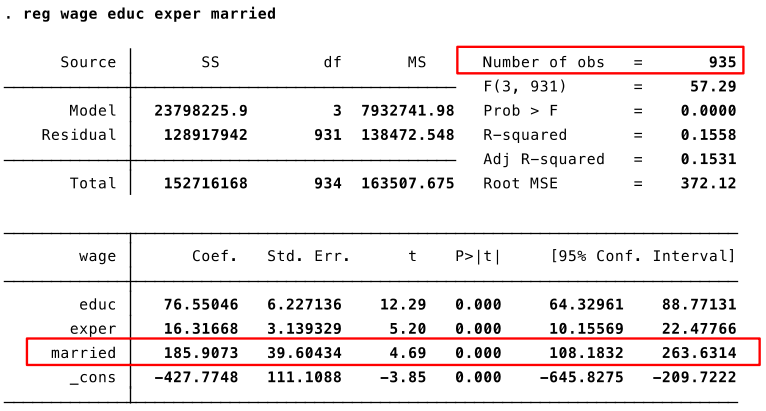
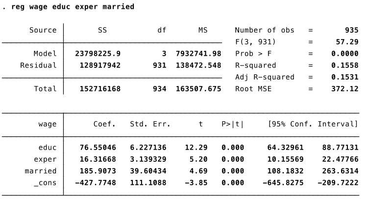
Example: Marriage premium

What is the effect of being married on wage?

Let’s estimate the following model: $$ wage = \beta_0 + \beta_1 educ + \beta_2 exper + \color{red}{\beta_3} married + u $$

Where married is a dummy variable which is 1 if the individual is married and 0 otherwise.
(We will talk more about dummy variables later)

Before we look at the data...

• Do we expect an effect?
  • Maybe marriage makes men more productive (married men may work harder, control their temper better, etc.).
• How large would such an effect be?
• Are there reasons why we believe OLS estimates might be biased?
  • Omitted Variable Bias: Maybe married men have other unobserved characteristics (intelligence, skill, etc.) that make them more productive.

Interpretation of OLS output

• Are MLR 1-4 true? Probably not.
• Is MLR 5 true? In practice, we use robust standard errors and don’t worry about this question for now. (We will talk about this later.)

• Is the sample large enough? Yes, so we don’t worry about MLR 6.

• My interpretation of the results:

  • The wage difference between married and not married men conditional on education and experience is statistically significant (i.e., it is most likely not a result of chance).
  • Because of likely omitted variable bias we can’t say anything about the causal effect of marriage on wage.

Remember how to interpret OLS coefficients.

Economic vs. statistical significance

• As we have seen, the statistical significance of a variable $x_j$ is determined by the size of the coefficient and size of the standard error.
• The economic significance of a variable is related to the size (and sign) of the estimated coefficient.
• Too much focus on statistical significance can lead to the false conclusion that a variable is ”important” even though the estimated effect is small.
• It is always important to interpret the magnitude of the estimated coefficient (in addition to looking at the statistical significance).

Guidelines for discussing economic & statistical significance

Nice discussion in Section 4.2 in the book. Summary:

• Check statistical significance. If significant, discuss the size of the estimated coefficient.
• If not significant at (at least) 10% level, check if the sign of the coefficient is in accordance with your expectation.
• There is nothing wrong with getting insignificant results.
• If the sign is the opposite to what you expect and the effect is statistically significant, this suggests that something isn’t quite right: perhaps your empirical specification (omitted variables?) or your underlying theory.

Emerging Best Practice

• Focus on point estimate and confidence intervals.

• Why confidence intervals? They tell us if 'big' or 'small' values/effects are plausible given the evidence.

• Don't focus on statistical significance at a specific cut-off level (95%, 99%, etc.)

• Report results for hypothesis tests for statistical significance using p-values.
  Big advantage is you can use p-value approach without needing to know the underlying distribution. E.g., we saw p-values in both t-test and F-test.

• There are some important exceptions: e.g., in most countries pharmaceutical regulation means drugs can be sold as treating a certain disease if their effect is shown to be statistically significant (non-zero), even if that effect might be small.

Review/Other

Hypothesis testing, old school

Today, any statistical program reports p-values.

In the past, researchers did hypothesis testing by looking up critical values in statistical tables.

While this is now hardly done in practice this approach is of some historical importance.

You don’t need to do this in the exam.