Quan 201: Multiple Regression Analysis
- Motivation
- Multiple Regression Model
- OLS estimator
- Measure of Goodness-of-Fit: R-squared
- OLS assumptions
- Omitted Variable Bias
- Variance of OLS estimator
Reference: Wooldridge "Introductory Econometrics - A Modern Approach", Chapter 3
Recap
- Outcomes of interest are determined by many factors.
- We are usually interested in the effect of one particular factor.
- $y=\beta_0+\beta_1 X_1 + \beta_2 X_2 + ...+ \beta_k X_k$
- $ y=\beta_0+\beta_1 X_1 + u $, where $u$ is all other factors.
OLS only gives an unbiased estimate of $\beta$ if $E[u|x] = E[u]$, which is often unrealistic (unless we have data from an experiment).
Example where E(u|x) = E(u) fails
- What is the effect of school expenditures on student test scores?
$$ Avg. \,Test\, scores =\beta_0+\beta_1 avg. \, expend + \beta_2 avg. \, income + u $$
- $\beta_2 \neq 0$
- $Corr(avg. \, income, avg. \, expend) \neq 0$
- In the US, schools in are locally funded so suburbs with high average income collect more taxes and can thus have higher expenditures. (By contrast, NZ national government funds all schools.)
Multiple Regression Analysis
We might have data on some of the other factors that affect the outcome.
Multiple regression analysis enables us to include more than one explanatory variable in our model.
By including more variables, we hold these variables explicitly constant.
This brings us closer to the ceteris paribus (all other things being equal) analysis than simple regression.
The model with k independent variables
$$y=\beta_0+\beta_1 X_1 + \beta_2 X_2 + ...+ \beta_k X_k + u$$
- $\beta_0$ is the intercept.
- $\beta_1$ shows the change in $y$ with respect to $x_1$.
- $\beta_2$ shows the change in $y$ with respect to $x_2$.
- (etc. for the other $\beta$ up to $\beta_k$)
- $u$ is the error term. It captures the effect of factors other than $x_1$,$x_2$,...,$x_k$ affecting $y$.
This framework can also be used to generalize the functional form (we will talk about this later).
We basically now mention more factors of the DGP explicitly!
OLS fitted values and residuals
For observation $i$ the fitted value or predicted value is simply $$ \hat{y}=\hat{\beta}_0+\hat{\beta}_1 X_1 + \hat{\beta}_2 X_2 + ...+ \hat{\beta}_k X_k$$
The residual for observation $i$ is defined just as in the simple regression case: $$ \hat{u}_i = y_i - \hat{y}_i$$
Question for Class
- Consider the following OLS estimates: $$\widehat{testscore}=\underbrace{88}_{\hat{\beta}_0} + \underbrace{1}_{\hat{\beta}_1}*classsize + \underbrace{6}_{\hat{\beta}_2}*ability$$
Consider Amanda:
- Testscore = 100
- Class size = 20
Ability = 2
What is Amanda’s predicted testscore?
- What is Amanda’s residual?
- What is Amanda’s error (u)?
Obtaining OLS estimates
OLS estimates: $$ \hat{y}=\hat{\beta}_0+\hat{\beta}_1 X_1 + \hat{\beta}_2 X_2 + ...+ \hat{\beta}_k X_k$$
OLS chooses $\hat{\beta}_0$, $\hat{\beta}_1$, $\hat{\beta}_2$,...,$\hat{\beta}_k$ to minimise the sum of squared residuals.
$$ \sum_{i=1}^n \hat{u}_i^2 = \sum_{i=1}^n (y_i-\hat{\beta}_0-\hat{\beta}_1 x_{i1} - \hat{\beta}_2 x_{i2}- ...- \hat{\beta}_k x_{ik}) ^2$$
Example: The FOC for $\hat{\beta}_1$
The minimization problem: Choose $\hat{\beta}$ so as to minimize: $$ \sum_{i=1}^n (y_i-\hat{\beta}_0-\hat{\beta}_1 x_{i1} - \hat{\beta}_2 x_{i2}- ...- \hat{\beta}_k x_{ik}) ^2$$ One part of this will be taking the partial derivative w.r.t. $\hat{\beta}_1$ and setting that equal to zero, this gives the FOC (first order condition) for $\hat{\beta}_1$. Namely,
$$ \sum_{i=1}^n x_{i1}(y_i-\hat{\beta}_0-\hat{\beta}_1 x_{i1} - \hat{\beta}_2 x_{i2}- ...- \hat{\beta}_k x_{ik})=0$$
[Technical note: there is a 2 that multiplies this, but we can simplify be cancelling it.]
Full FOCs: k+1 equations for k+1 unknowns
Taking the FOCs for each element of $\hat{\beta}$ we get the system of equations:
$$ \sum_{i=1}^n (y_i-\hat{\beta}_0-\hat{\beta}_1 x_{i1} - \hat{\beta}_2 x_{i2}- ...- \hat{\beta}_k x_{ik})=0$$
$$ \sum_{i=1}^n x_{i1}(y_i-\hat{\beta}_0-\hat{\beta}_1 x_{i1} - \hat{\beta}_2 x_{i2}- ...- \hat{\beta}_k x_{ik})=0$$
$$ \sum_{i=1}^n x_{i2}(y_i-\hat{\beta}_0-\hat{\beta}_1 x_{i1} - \hat{\beta}_2 x_{i2}- ...- \hat{\beta}_k x_{ik})=0$$
$$ \vdots $$
$$ \sum_{i=1}^n x_{ik}(y_i-\hat{\beta}_0-\hat{\beta}_1 x_{i1} - \hat{\beta}_2 x_{i2}- ...- \hat{\beta}_k x_{ik})=0$$
Solving these is simple, but tedious. (Much easier using matrices and vectors.)
We will never actually do this. Computer calculates the solution for us.
Sample properties of OLS estimator
$$ \sum_{i=1}^n (y_i-\hat{\beta}_0-\hat{\beta}_1 x_{i1} - \hat{\beta}_2 x_{i2}- ...- \hat{\beta}_k x_{ik})=0$$
$$ \sum_{i=1}^n x_{i1}(y_i-\hat{\beta}_0-\hat{\beta}_1 x_{i1} - \hat{\beta}_2 x_{i2}- ...- \hat{\beta}_k x_{ik})=0$$
$$ \sum_{i=1}^n x_{i2}(\underbrace{y_i-\hat{\beta}_0-\hat{\beta}_1 x_{i1} - \hat{\beta}_2 x_{i2}- ...- \hat{\beta}_k x_{ik}}_{residual, \, \hat{u}_i})=0$$
$$ \vdots $$
$$ \sum_{i=1}^n x_{ik}(y_i-\hat{\beta}_0-\hat{\beta}_1 x_{i1} - \hat{\beta}_2 x_{i2}- ...- \hat{\beta}_k x_{ik})=0$$
From the FOCs it follows that:
- Average value and sum of $\hat{u}_i$'s are equal to zero.
- Covariance of each variable, e.g. $x_3$, with $\hat{u}$ is equal to zero.
Note: this is mechanically so because of the way OLS is estimated and does not say anything about the unobserved error term $u$.
Interpretation of equation with k independent variables
The coefficient on $x_1$ ($\hat{\beta}_1$) measures the change in $\hat{y}$ due to a one-unit increase in $x_1$, holding all other independent variables fixed: $$ \Delta \hat{y} = \hat{\beta}_1 \Delta x_1 $$
Partialling out interpretation of $\hat{\beta}_j$
$$\hat{\beta}_j=\frac{Cov(y,\tilde{x}_j)}{Var(\tilde{x}_j)}$$ Where $\tilde{x}_j$ are the residuals of a regression of $x_j$ on all the covariates ($x_1$,...$x_{j-1}$,$x_{j+1}$,...,$x_k$)
- $\hat{\beta}_j$ measures the sample relationship between $y$ and $x_j$ after all the other covariates have been partialled out.
(Also use wording 'after controlling for')
[Note: At first glance the above formula looks different to the textbook but it is the same equation.]
[Intuition: $\tilde{x}_j$ is the part of $x_j$ which cannot be accounted for by the other covariates; hence it is the residuals of regression of $x_j$ on the other covariates.]
Goodness-of-fit:
Same as for simple regression model
- SST = Total Sum of Squares
- SSE = Explained Sum of Squares
- SSR = Residual Sum of Squares
$$ SST = \sum_{i=1}^n (y_i-\bar{y})^2 \quad SSE = \sum_{i=1}^n (\hat{y}_i - \bar{y})^2 \quad SSR = \sum_{i=1}^n (\hat{u}_i)^2 $$
$$ SST=SSE + SSR$$
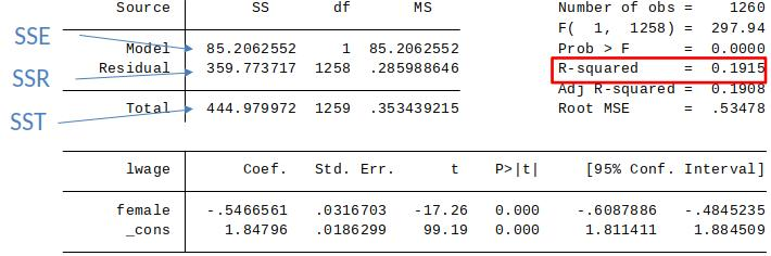
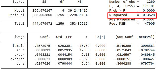
$$ R^2=\frac{SSE}{SST}=1-\frac{SSR}{SST}$$
R-squared
The R-squared never decreases, and usually increases, when another independent variable is added to a regression.
This is because the SSR can never increase when you add more regressors to the model (why?)
Simple Regression:
From World 2 to World 1
The discussion above was about properties of the OLS estimator that hold in any dataset (world 2).
Now we discuss under which circumstances OLS estimates tell us something about the DGP (world 1).
Remember, if the expected value of the OLS estimator is equal the true parameter (from world 1) our OLS estimator is unbiased ($E[\hat{\beta}_j]=\beta_j$)
From World 2 to World 1 (cont.)
The multiple linear regression (MLR) assumptions are mostly straightforward extensions of those we saw for the simple regression model.
MLR 1. – 4. describe the conditions under which OLS gives us unbiased estimates of the underlying population model.
Assumptions
Assumption MLR.1: Linear in parameters: $$y=\beta_0+\beta_1 X_1 + \beta_2 X_2 + ...+ \beta_k X_k + u$$
Assumption MLR.2: Random sampling:
We have a random sample of n observations of $\{(x_{i1}, x_{i2},...,x_{ik},y_i): \, i=1,2,...,n\}$
Assumption MLR.3: No perfect collinearity:
In the sample, none of the independent variables is constant and there are no exact linear relationships among the independent variables.
Assumption MLR.4: Zero conditional mean:
The error u has an expected value of zero given any values of the independent variables:
$E[u|x_1, x_2,…,x_k]=0$
MLR. 1-3
We will talk about MLR. 1 later.
Assumption MLR. 2 is straightforward.
Assumption MLR.3 is new: No perfect collinearity.
Key in practice: No exact linear dependence between independent variables.
If there is linear dependence between variables, then we say there is perfect collinearity. In such a case we cannot estimate the parameters using OLS.
Examples:
$x_2 = 4*x_1$
$x_3 = 5*x_1 + 7*x_2$
Example of perfect collinearity
This type of model can’t be estimated by OLS: $$ cont = \beta_0 + \beta_1 IncomeInDollars + \beta_2 IncomeInThousandsOfDollars + u$$ since $IncomeInThousandsOfDollars=1000*IncomeInDollars$ there is linear dependence.
However, this type of model can be estimated by OLS: $$ cont = \beta_0 + \beta_1 Income+ \beta_2 Income^2 + u$$ while $Income$ and $Income^2$ are related, they are not linearly related.
MLR.4: Zero conditional mean
MLR.4 $E(u|x_1, x_2,...,x_k)=0$ is a direct extension of SLR.4.
It is the most important of the four assumptions MLR.1-4, and implies that the error term u is uncorrelated with all explanatory variables in the population.
When MLR.4 holds, we sometimes say that the explanatory variables are exogenous.
Why MLR.4 may fail
MLR.4 may fail for the following reasons:
- Omitting an explanatory variable that is correlated with any of the $x_1, x_2,...,x_k$.
- Misspecified functional relationship between the dependent and independent variables. (We will talk more about this later)
The first of these – omitted variables – is by far the biggest concern in empirical work.
Towards a weaker version of MLR 4
What is the effect of attending a private university?
Motivation: private selective university (e.g. Harvard, Yale) are more expensive compared to public universities (e.g., University of Texas). Do they lead to higher earnings later in life?
Problem: students who go to private selective universities are different from those who go to public colleges (selection bias).
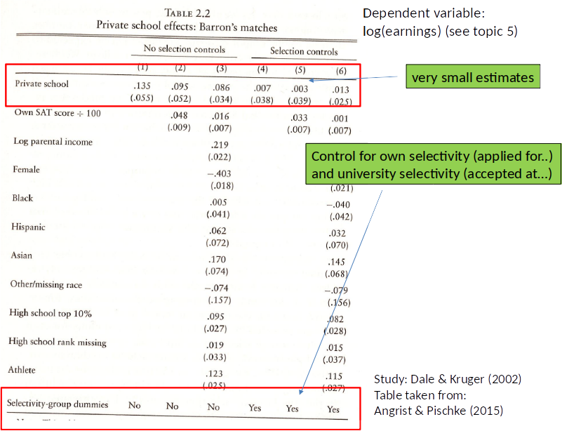
Return to Private University
Dale and Kruger (2002) have data on students who graduated in 1972 including earnings later in life.
This data also includes information on which institutions the student applied to and at which institutions they were accepted.
Consider the following model:
$$wage = \beta_0 + \beta_1 private + \gamma_1 applied private + \gamma_2 accepted private + \gamma_3 SAT score+ u$$
where
$private=1$ if went to private university, 0 otherwise.
$appliedprivate=1$ if applied to private university, 0 otherwise.
$acceptedprivate=1$ is accepted at private university, 0 otherwise.
$SAT score=$ students score on SAT test
- Do people who applied for and got accepted to the same colleges, with the same SAT score, differ systematically in other factors that affect wage?
Is:
$E[u|private,appliedprivate,acceptedprivate,SATscore]=E[appliedprivate,acceptedprivate,SATscore]$
Discuss.
[Note: SAT was a common test for university access at the time.]
Weaker version of MLR 4
Consider the following model:
$$y=\beta_0 + \beta_1 P + \gamma_1 x_1 + \gamma_2 x_2 +... \gamma_k x_k + u$$
where:
$P=$ variable of interest.
$\beta_1=$ parameter of interest.
$x_1,x_2,...,x_k=$ variables not of interest (control variables).
$\gamma_1, \gamma_2,..., \gamma_k=$ parameters not of interest.
OLS leads to unbiased estimates of causal effect of $\beta_1$ (but not $\gamma_1, \gamma_2,..., \gamma_k$) if: $$E[u|P,x_1,...,x_k]=E[u|x_1,...,x_k]$$
In words: if the average value of the error term $u$ in the population, when holding constant $\gamma_1, \gamma_2,..., \gamma_k$ is the same for all values of $P$.
Weaker MLR 4: intuition
$$y=\beta_0 + \beta_1 P + \gamma_1 x_1 + \gamma_2 x_2 +... \gamma_k x_k + u$$
Ask yourself:
Holding observed other factors ($\gamma_1, \gamma_2,..., \gamma_k$) constant, is P unrelated to the unobserved other factors?
- If yes, OLS estimator of the effect of variable of interest $\beta_1$ is unbiased (i.e. $\hat{\beta}_1$ is unbiased)
- If no, OLS estimator of the effect of variable of interest $\beta_1$ is biased ($\hat{\beta}_1$ is biased)
Example 2: Gender Wage Gap
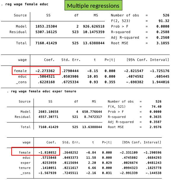
$$wage = \beta_0+\beta_1 female +\gamma_1 educ + \gamma_2 exper + \gamma_3 tenure + u$$
We are interested in $\beta_1$, which shows the causal effect of being female on wage.
We control for education, experience and tenure to make the comparison ceteris paribus. We do not care about their causal effect on wage.
Is $E[u|female, educ, exper, tenure]=E[u|educ, exper, tenure]$?
Or do women with the same years of education, experience and tenure differ systematically in unobserved factors that matter for wage ($u$) from men? Discuss.
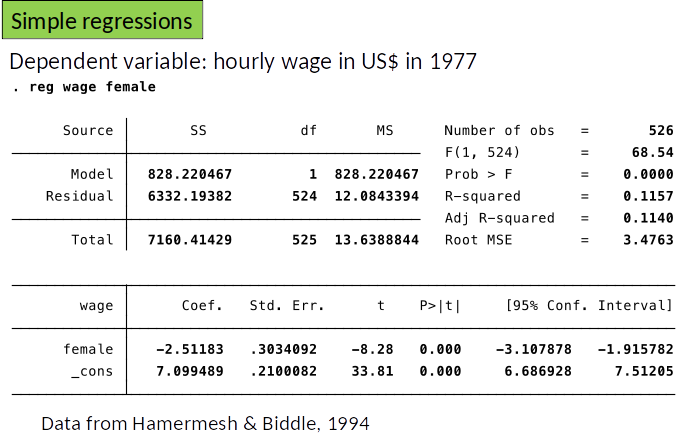
Interpretation: women earn on average $2.51 less per hour.
Gender wage gap
Even if $$E[u|female, educ, exper, tenure] \color{red}{\neq} E[u|educ, exper, tenure]$$
$\hat{\beta}_1$ is still interesting!
$\hat{\beta}_1$ shows us the average wage difference between men and women (in our sample) who have the same level of education, experience and tenure.
[Just that we cannot interpret it as causation.]
Omitted Variable Bias (OVB)
One main reason why MLR 4. fails is if we omit an important variable in the regression $\to$ OLS estimates will be biased.
(Note: We often still find the relationship in the data interesting (world 2)).
We might be able to deduce in which direction the OLS is biased and thus learn if our OLS estimate is likely larger or smaller than the true effect.
We can do this by thinking carefully how the OLS estimates would look like if we were to include the omitted variable.
OVB:
OVB: Simple case
Let’s first look what happens mechanically (in world 2) if we omit a variable.
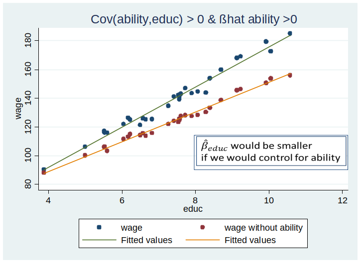
Suppose we are interested in the effect of education on wage.
How would the regression line look like if we could partial out the effect of ability?
OVB formula: simple case
- Simple regression: $\tilde{y}=\tilde{\beta}_0 +\tilde{\beta}_1 x_1$
- Multiple regression: $\hat{y}=\hat{\beta}_0 +\hat{\beta}_1 x_1 +\hat{\beta}_2 x_2$
We know that the simple regression coefficient will be: $$\tilde{\beta}_1=\hat{\beta}_1 + \hat{\beta}_2 \tilde{\delta}_1$$
where $\tilde{\delta}_1$ is the slope coefficient from a simple regression of $x_2$ on $x_1$. How can this be understood?
- Simple regression: $\tilde{y}=\tilde{\beta}_0 +\tilde{\beta}_1 x_1$
- Multiple regression: $\hat{y}=\hat{\beta}_0 +\hat{\beta}_1 x_1 +\hat{\beta}_2 x_2$ $$\tilde{\beta}_1=\hat{\beta}_1 + \hat{\beta}_2 \tilde{\delta}_1$$
So, the estimates of $\beta_1$, namely $\hat{\beta}_1$ and $\tilde{\beta}_1$ are the same if the second term, $\hat{\beta}_2 \tilde{\delta}_1$ is zero; i.e., if...
- The partial effect of $x_2$ on $\hat{y}$ is zero in the sample ($\hat{\beta}_2=0$).
$ and/or $ - $x_1$ and $x_2$ are uncorrelated in the sample ($\tilde{\delta}_1=0$).
OVB: simple case
The formula $\tilde{\beta}_1=\hat{\beta}_1 + \hat{\beta}_2 \tilde{\delta}_1$ holds always in the data (World 2).
In the special case where $\hat{\beta_1}$ and $\hat{\beta_2}$ are unbiased (i.e., MLR 1. – 4. would hold if we could include/observe $x_1$ and $x_2$), the bias is $\tilde{\beta}_1$ is given by, $$ Bias(\tilde{\beta}_1)=\beta_2 \delta_1$$
Note: define $Bias(\hat{\beta})=E[\hat{\beta}]-\beta$.
Signing Bias
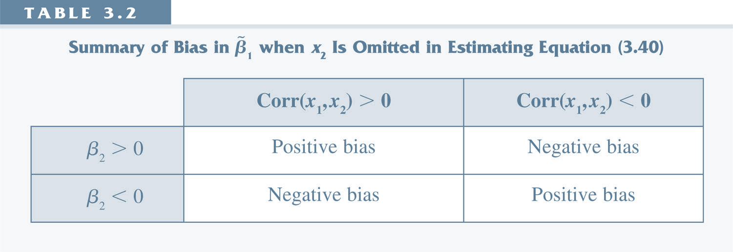
Note: this shows only the bias in the case where a regression with $x_1$ and $x_2$ would have been unbiased. However, the table can still be used to learn how $\hat{\beta}_1$ and $\tilde{\beta}_1$ differ (in world 2).
Omitted variable bias: More general cases
- Deriving the sign of omitted variable bias when there are multiple regressors in the estimated model is more difficult.
- In general, correlation between a single explanatory variable and the error results in all estimates being biased.
Homoskedasticity (MLR 5)
Assumption MLR.5: Homoskedasticity.
The error $u$ has the same variance given any value of the explanatory variables:
$$Var(u|x_1,x_2,...,x_k)=\sigma^2$$
This means that the variance in the error term $u$ conditional on the explanatory variables, is the same for all values of the explanatory variables.
If this is not the case, there is heteroskedasticity and the formula for the variance of $\beta_j$ has to be adjusted. We will talk about this later.
Variance of the OLS estimator
Under assumptions MLR.1-5 (also known as the Gauss-Markov assumptions):
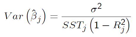
$SST_j=\sum_{i=1}^n (x_{ij}-\bar{x}_j)^2$ is the total sum of squares of $x_j$
$R_j^2$ is the R-squared from regressing $x_j$ on all other regressors (and including an intercept).
Interpreting the variance formula
The variance of the estimator is high (which is typically undesirable) if...
- The variance of the error term is high.
- The total sampling variance of the $x_j$ is low (e.g. due to low variance or small sample).
- The $R_j^2$ is high. Note that, as $R_j^2$ gets close to 1 – due to near linear dependence amongst regressors (multicollinearity) – the variance can become very large.
Estimator of Variance of $\hat{\beta}_j$
We already saw that $$Var(\hat{\beta}_j) = \frac{\sigma^2}{SST_j (1-R_j^2)}$$ but we don't observe $\sigma^2$, so we cannot just use this.
To get an estimator of $Var(\hat{\beta}_j)$ we replace the true (and unobserved) parameter $\sigma^2$ with $\hat{\sigma}^2$, which is an estimator of $\sigma^2$. $$ \hat{\sigma}^2 = \frac{\sum_{i=1}^n \hat{u}_i^2}{n-k-1} = \frac{SSR}{n-k-1}$$ and the resulting estimator is $$\widehat{Var}(\hat{\beta}_j)=\frac{\hat{\sigma}^2}{SST_j (1-R_j^2)}$$
Estimating standard errors of the OLS estimates
The main practical usage of the variance formula is for calculating standard errors of the OLS estimates. Standard errors are estimates of the standard deviation of $\hat{\beta}_ j$
Recall that the standard deviation (sd) is equal to the square root of the variance. $$ sd(\hat{\beta}_j) = \sqrt{Var(\hat{\beta}_j)} $$
The standard error is simply the square root of the estimator of the variance of . $$ se(\hat{\beta}_j) = \sqrt{\widehat{Var}(\hat{\beta}_j)} $$
Standard error (cont.)
$$ se(\hat{\beta}_j) = \sqrt{\widehat{Var}(\hat{\beta}_j)} $$
$$ se(\hat{\beta}_j) = \sqrt{\frac{\hat{\sigma}^2}{SST_j (1-R_j^2)}}$$
The standard error is large (which is typically undesirable) if...
- SSR is high
- The total sampling variance of the $x_j$ is low (e.g. due to low variance or small sample).
- The $R_j^2$ is high.
We use standard errors for hypothesis testing – more on this in topic 4.
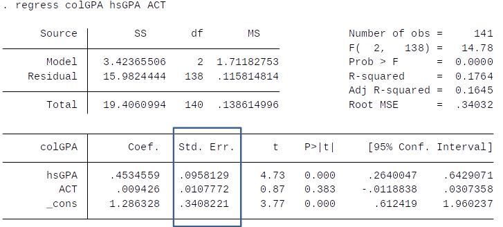
Standard errors in Stata
Efficiency of OLS: The Gauss-Markov Theorem
- Under assumptions MLR.1-5, OLS is the Best Linear Unbiased Estimator (BLUE) of the population parameters.
- Best = smallest variance
- It’s reassuring to know that, under MLR.1-5, you cannot find a better estimator than OLS.
- If one or several of these assumptions fail, OLS is no longer BLUE.