OLS Regression
- Data Generating Process (DGP)
- Econometric model
- Simple Linear Regression Model
- Deriving the Ordinary Least Squares (OLS) Estimator
- Sampling distribution of OLS estimator
- Variance of OLS estimator
- OLS assumptions
- Measure of Goodness-of-Fit: R-squared
Reference: Wooldridge "Introductory Econometrics - A Modern Approach", Chapter 2
What is the effect of reducing class size on student outcomes?

What is the effect of reducing class size on student outcomes?
- Which outcome do we care about?
- Student happiness?
- Student learning?
- Etc.
- Let’s use test score as measure of student learning.
Data Generating Process (DGP)
As social scientists, we fundamentally believe that there is something to be learnt by treating the world as orderly and predictable.
We believe that test scores (and all other outcomes) are generated by a predictable process. We call this process the Data Generating Process (DGP).
Before looking at the data, we should think about the DGP.
Thinking about the test score DGP
- Test score (Y) is generated by some process.
- Which factors (Xs) influence student test scores?
- Class size
- Ability
- Motivation
- Household income
- Etc.
Econometric model
- An Econometric model is a mathematical description of the DGP.
- Consider the following econometric model that describes how the test scores are generated: $$ Test Score = \beta_0 +\beta_1 X_1 + \beta_2 X_2 + ...+ \color{red}{\beta_{cs}\textit{class size}}+... +\beta_k X_k $$
- We are typically interested in the effect of one particular factor on the outcome; in our case class size.
- Much of Econometrics is about estimating $\beta$ (pronounced 'beta').
The $\beta$ coefficient
- $\beta$ shows how change in one factor affects the outcome
$$ \beta_{cs} = \frac{\textit{change in test score}}{\textit{change in class size}} = \frac{\Delta\textit{test score}}{\Delta\textit{class size}} $$ therefore $$ \Delta \textit{test score} = \beta_{cs} \Delta\textit{class size}$$
If we would increase class size by one, holding all the other factors constant, test scores will change by $\beta_{cs}$.
$\beta_{cs}$ shows the causal effect of a change in class size. (Under assumptions of DGP)
Simple Linear Regression (SLR) Model
$$Test scores = \beta_0 + \beta_{cs}* class size + other factors$$
More general: $$y=\beta_0 + \beta_1 X + u$$ call $\beta_0$ the intercept parameter or constant call $\beta_1$ the slope
Hypothetical DGP: $$ testscore=\underbrace{100}_{\beta_0} -\underbrace{0.5}_{\beta_1}*class size + \underbrace{5*ability -5*lazy}_{u} $$
Note that in real life we almost never know all the factors that influence an outcome.
Question for Class
Consider the following hypothetical DGP: $$ testscore=100 -0.5*class size + 5*ability -5*lazy$$
Consider Amanda:
- class size = 20
- ability = 2
- lazy = 1
What is Amanda’s testscore?
By how much will Amanda’s testscore change if the class size increases to 21 students?
Ordinary Least Squares (OLS)
OLS is a statistical method which gives us the line (called sample regression function (SRF) wich minimizes the squared distance from the points (observations) to the regression line.
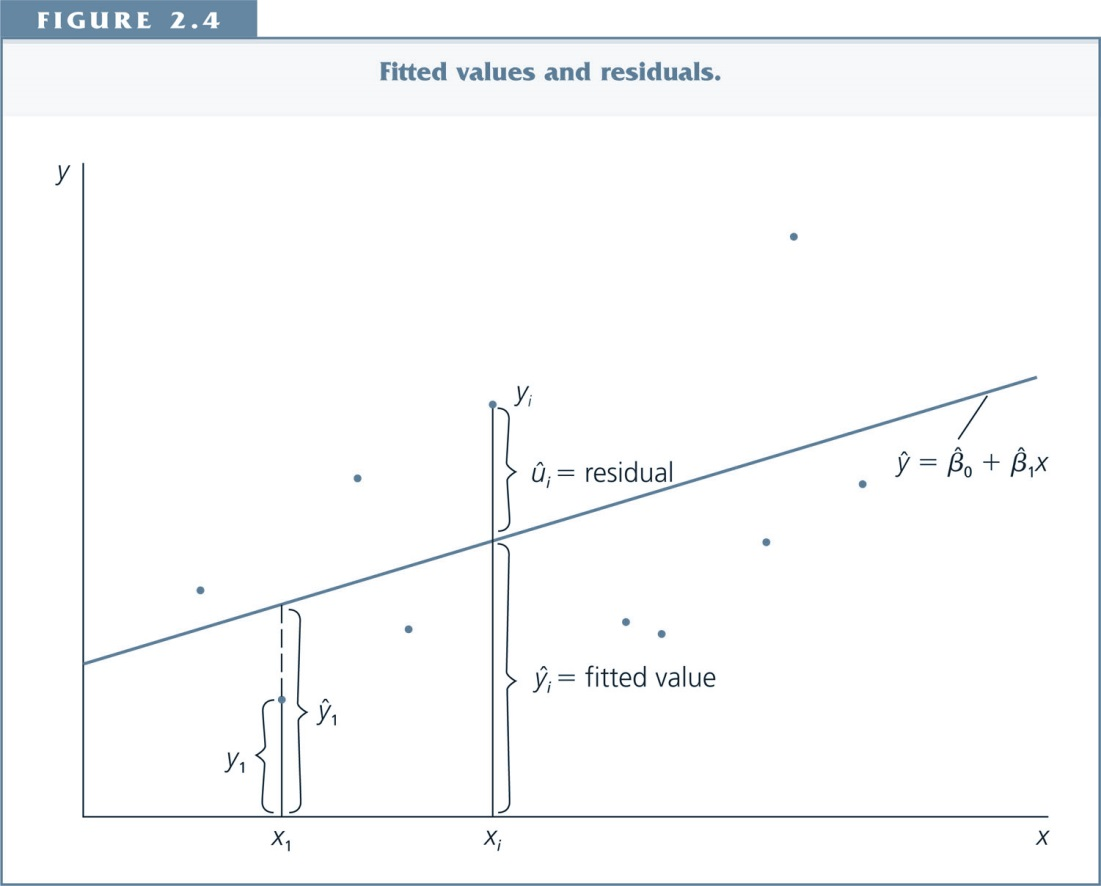
Let's decompose $y_i$
Actual Observation: $y_i=\hat{\beta_0}+\hat{\beta_1} x_i + \hat{u_i}$
Predicted value/fitted value: $\hat{y}_i=\hat{\beta_0}+\hat{\beta_1} x_i$
Residual: $\hat{u_i}=y_i-\hat{y_i}$
(Residual=Difference between actual and predicted value)
OLS Estimators
How does OLS minimize the sum of squared residual? $$ \sum^n_{i=1} \hat{u}_i^2 = \sum^n_{i=1} (y_i-\hat{\beta}_0-\hat{\beta}_1 x_i)^2 $$
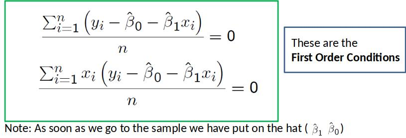
Set the first derivatives with respect to $\hat{\beta}_0$ and $\hat{\beta}_1$ equal to zero.
Then you get these First Order Conditions: $ \quad \sum^n_{i=1} (y_i-\hat{\beta}_0-\hat{\beta}_1 x_i)=0$ and $ \quad \sum^n_{i=1} x_i(y_i-\hat{\beta}_0-\hat{\beta}_1 x_i)=0$
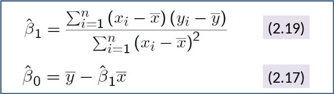
Which you can solve to get: $ \quad \hat{\beta}_1=\frac{Cov(x,y)}{Var(x)}$ and $\hat{\beta}_0=\bar{y}-\hat{\beta}_1 \bar{x}$
where $\bar{y}$ and $\bar{x}$ are the mean of $y$ and $x$ respectively.
Review of important statistical concepts
Mean
$\mu_x$ = population mean = mean (average) of all observations in a population. Note that $\mu_x= E(x)$. $$\mu_x = \frac{\sum^N_{i=1} x_i}{N}$$
$\bar{x}$ = sample mean = mean (average) of all observations in a sample. Estimator of population mean $$\bar{x} = \frac{\sum^n_{i=1} x_i}{n}$$
$n$ is the number of observations in the sample. ($N$ would often be infinite, in which case the sum is an integral.)
Pronunciation: $\mu$ is 'mu' or 'mew'. $\bar{x}$ is 'x bar'.
Variance
$Var(x)$: The variance is a measure of how far a set of numbers is 'spread out'. How much they vary.
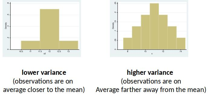
[Notice the scales of the x-axes]
Variance
$\sigma_x^2$ = population variance = variance of all observations in a population. $$\sigma_x^2 = \frac{\sum^N_{i=1} (x_i-\mu_x)^2}{N}$$
$S^2$ = sample variance = estimator of population variance. $$S^2 = \frac{\sum^n_{i=1} (x_i-\bar{x})^2}{n-1}$$
Pronunciation: $\sigma^2$ sigma squared.
Covariance
The Covariance is a measure of how much two variables change together.
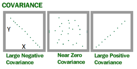
Human height and weight has a positive covariance.
Weather and day of the week has a zero covariance.
Covariance
$\sigma(X,Y)$ = Population Covariance between X and Y.
$$\sigma(X,Y)= \frac{\sum^{N}_{i=1} (x_i-\mu_x)(y_i-\mu_y)}{N}$$
$Cov(X,Y)$ = Sample Covariance between X and Y.
$$Cov(X,Y)= \frac{\sum^{n}_{i=1} (x_i-\bar{x})(y_i-\bar{y})}{n-1}$$
Covariance and Correlation
The (Pearson product-moment) correlation coefficient is a standardized covariance.
The correlation always has the same sign as the covariance, but it is transformed to be between -1 and 1.
(Covariance is measured in the units of X and Y, correlation avoids this.)
Estimate Simple Regression by Hand
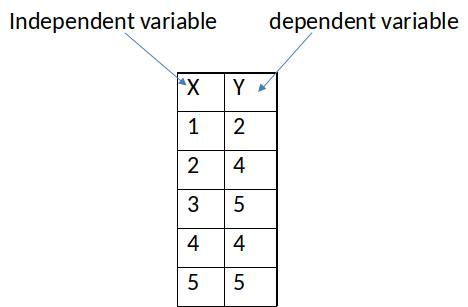
What is the line that minimizes the sum of squared residuals?
To get this line, we need the slope ($\beta_1$) of the line and the constant ($\beta_0$).
$\hat{\beta}_1=\frac{Cov(x,y)}{Var(x)}$ and $\hat{\beta}_0=\bar{y}-\hat{\beta}_1 \bar{x}$
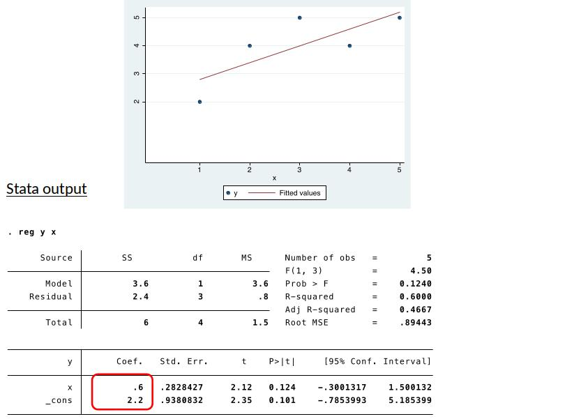
Estimate Simple Regression in Stata
Sample properties of OLS
$\sum_{i=1}^n (\underbrace{y_i-\hat{\beta}_0-\hat{\beta}_1 x_i}_{residual})=0$ $\quad \quad \to$ sample average (and sum) of the residuals ($\hat{u}_i$) is zero.
$\sum_{i=1}^n x_i(\underbrace{y_i-\hat{\beta}_0-\hat{\beta}_1 x_i}_{residual})=0$ $\quad \to$ sample covariance of $x$ and $\hat{u}$ is zero.
$\hat{\beta}_0=\bar{y}-\hat{\beta}_1 \bar{x}$ $\quad \quad \quad \quad \quad \quad \to$ The point ($\bar{x}$,$\bar{y}$) is on the regression line (SRF).
$\hat{\beta}_1=\frac{Cov(x,y)}{Var(x)}$ $\quad \quad \quad \quad \quad \quad \to$ $\hat{\beta_1}$ has the same sign as the sample covariance of $x$ and $y$.
These properties hold in any/every sample!
A tale of two worlds
World 1: The model world (DGP world)
- Describes the process that generates the data (e.g., $y=\beta_0+\beta_1+u$)
- Is unobserved
- The parameters of the slope coefficients (e.g., $\beta_1$) indicate the causal effects of a variable (hence Data Generating Process)
- We usually describe the parameters of the model using greek letters (without hat)
World 2: The sample world
- Is about the relationship between variables in the sample (with actual data)
- Is observed.
- We use greek letters with hat to refer to empirical relationships between variables(e.g., $\hat{\beta}_1$)

OLS estimators
In econometrics we usually want to learn about World 1 (DGP) by looking at data.
Because of this, we refer to the constant ($\hat{\beta}_0$) and slope coefficient ($\hat{\beta}_1$) from world 2 as estimators. They are estimators of the unobserved parameters.
$\hat{\beta}_0$ and $\hat{\beta}_1$ are only in very particular circumstances “good” estimators of $\beta_0$ and $\beta_1$. I.e., they often don’t tell us much about the DGP.
However, $\hat{\beta}_1$ is often still interesting because it tells us about the relationship between X and Y in our data (even if we cannot interpret $\hat{\beta}_1$ causally).
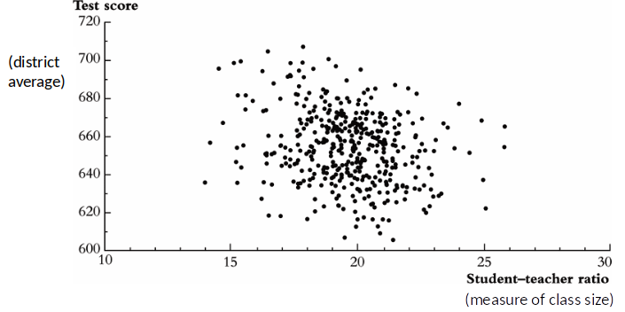
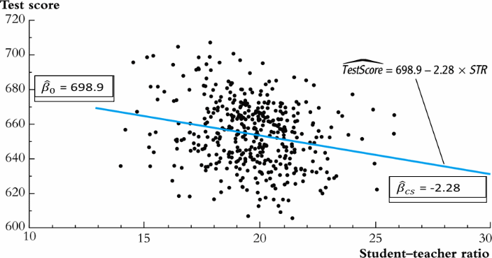
What can we learn from OLS?
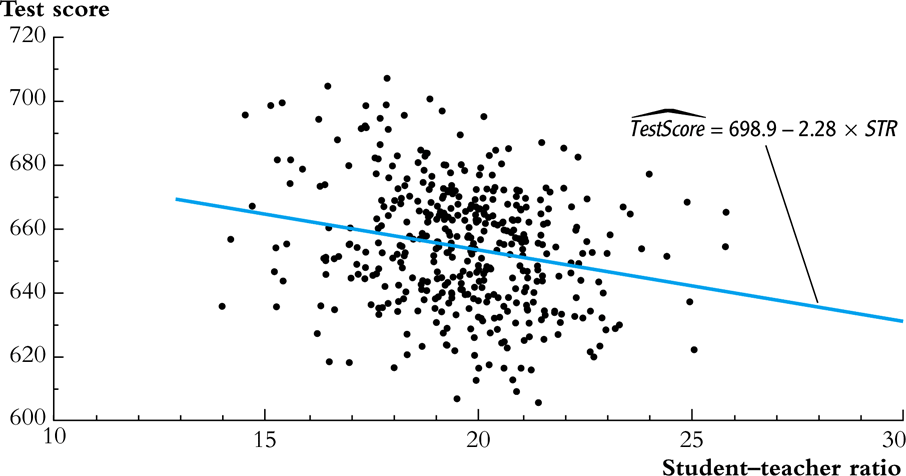
$\hat{\beta}_{cs}$ shows us that districts that have higher student-teacher ratio (STR) have on average lower test scores. (There is a negative relationship between test score and class size.)
What does this tell us about the effect of reducing class size? Is the comparison between schools with high and low STRs ceteris paribus?
OLS Ceteris paribus
Only when all other relevant factors are equal (on average) we get a ”good” estimate of the causal effect of class size on test score using OLS.
All other factors are captured in the error term $u$.
For OLS ”ceteris paribus” means that $u$ is on average the same for all values of class size ($X$).
Students in districts with at STR (class size) of 15 have on average higher test socres than those in districts with a STR of 25.
What are the two potential reasons for that?
- Lower STR
- Everything else (captured in u)
What factors could be in u? student ability, motivation, teacher quality, etc.
Is u on average the same for classes with STR of 15 as for STR of 25?
Is u on average the same for all STRs? Discuss.
Intuitive explanation of OLS estimator
Let’s imagine three cases in the sample:
- u is equal to zero for all observations.
- u is on average equal to zero for all values of x.
- u is on average not equal to zero for all values of x.
Case 1: u = 0 for all students
DGP: $ testscore=100 -0.5*class size + 5*ability -5*lazy$
- We only observe testscore and classize.
- We do not observe ability and lazy (the only two variables in the error term).
- We want to estimate the effect of classsize ($\beta_1=-0.5$) on testscore and the constant ($\beta_0=100$).
Case 1: u = 0 for all students (continuted)
DGP: $ testscore=100 -0.5*class size + 5*ability -5*lazy$
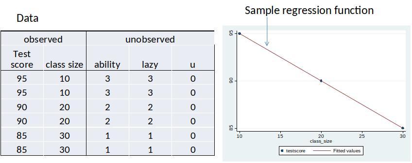
The sample regression function is $100 -0.5*class size$ (same as DGP)
All observations are on the line.
Case 2: u is on average equal for all values of x
DGP: $ testscore=100 -0.5*class size + 5*ability -5*lazy$
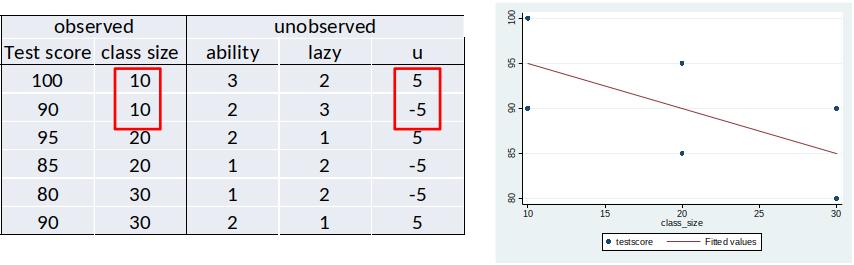
The sample regression function is equal to $100 -0.5*class size$ (but not all observations are on the line)
Intuition: If $u$ is on average 0 for all levels of $class size$, then $100 -0.5*class size$ minimizes the sum of squared residuals.
Case 3: u is on average not equal to zero for all values of x
DGP: $ testscore=100 -0.5*class size + 5*ability -5*lazy$
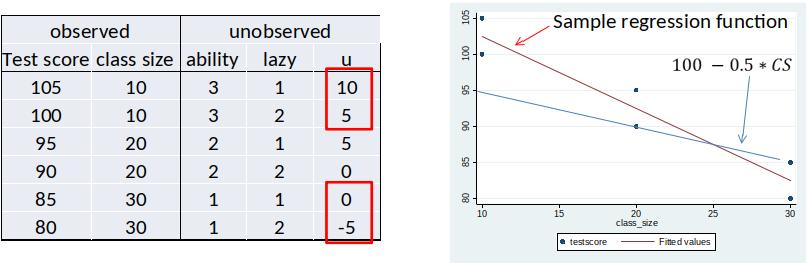
The sample regression function is not equal to $100 -0.5*class size$
Intuition: If u is on not average 0, $100 -0.5*class size$ then does not minimize the sum of squared residuals.
Ceteris Paribus?
Notice how, at the intuitive level we talked about $u$ as everything else. Analagous to what we discussed with taking the difference in group means when thinking about causation and experiments (in Topic 1) we might think that when 'everything else' averages to zero we can estimate what we are wanting to.
It turns out this is not quite enough. We need something more subtle. We need that 'everything else' is zero on average (in the population) for each value of x. When this is the case, we can estimate 'well'. (Accuracy coming with large samples.)
Let's make this idea more precise over the next bunch of slides...
From sample to population
- If $u$ is on average equal to zero for all values of $x$ in the sample, the OLS sample regression function will be exactly the DGP. But this is (effectively) never going to be the case in any specific sample.
- However, $u$ could be on average equal to 0 for all values of $x$ in the population.
- If this is true the OLS estimator is correct on average (if we would take many samples, and estimate many regressions).
- We call an estimator that is correct on average unbiased.
OLS assumption
Critical OLS assumption:
$$ E[u|x]=E[u] $$
- The left-hand side is a conditional expectation.
- The right-hand side is an unconditional expectation (just the expected value of u, regardless of x).
Interpretation: The average value of $u$ in the population is the same for all values of $X$. This is the equivalent of the ceteris paribus condition for OLS.
- If this assumption holds, OLS gives us a ”good” estimate of the causal effect.
Note: Wooldgridge talks about assumptions we have to make in order to get reliable estimates of $\beta_1$... You can think of this as conditions/circumstances that need to be true.
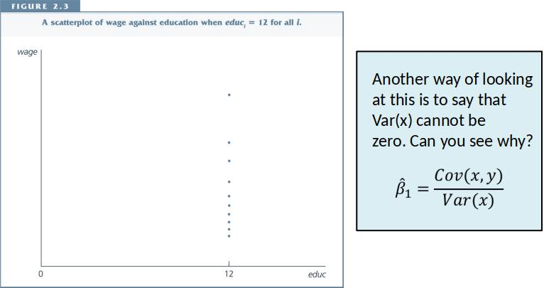
Conditional Expectation
Example:
- X is education and Y is hourly wage.
- $E(Y|X=12)$ is the average hourly wage for all people in the population with 12 years of education.
- $E(Y|X=16)$ the average hourly wage for all people in the population with 16 years of education
Illustration
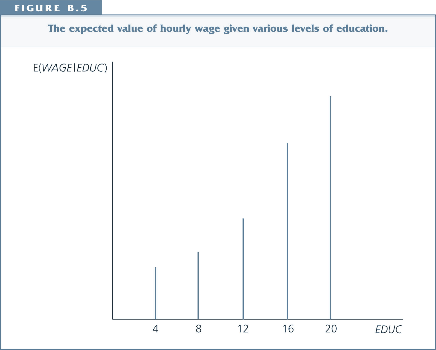
Illustration follow up question
How would you draw a figure of $E[u|x]$? (Similar to the previous one.)
How would the figure look if $E[u|x]=E[u]$?
Think about: What axes, and what would the values (the heights of the lines) be?
A Less Controversial Assumption
As long as the intercept $\beta_0$ is included in the equation, we can always assume that the average value of $u$ in the population is zero: $$E[u]=0$$ If in truth $E[u]\neq 0$ we get ”bad” estimates of $\beta_0$, but we are rarely interested in estimating $\beta_0$. So we will assume $E[u]=0$.
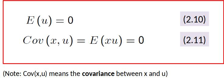
We combine $E[u|x]=E[u]$ and $E[u]=0$ to get the zero conditional mean assumption: $$ E[u|x]=0$$
From assumptions to estimators
Assumption: $E[u|x]=E[u]$
Assumption: $E[u]=0$
Both assumptions together imply zero covariance between x and u. We can now re-write the above assumptions as
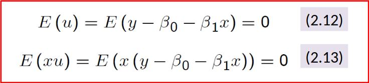
Note: $u=y-\beta_0-\beta_1 x$
Re-write the above assumptions again:
We have two unknown parameters. Can’t we just solve for these?
Not quite, because we don’t know the expected values of $y$ and $x$ in the population.
It’s precisely for this reason that the best we can hope to do is estimate the parameters.
(We will never be able to know the true population values of the parameters, only to estimate them.)
This applies for the population:
$\hat{\beta}_0$ and $\hat{\beta}_1$ miminize the sum of squared residuals.
We can rewrite ($2.19$) as follows: $\hat{\beta}_1=\frac{Cov(x,y)}{Var(x)}$
What just happened?
We got the same estimators for $\hat{\beta}_0$ and $\hat{\beta}_1$ as before.
The first time we got them it was from the OLS regression, they are the OLS regression estimators.
The second time we got them it was the assumptions $E[u|x]=E[u]$ and $E[u]=0$, they are the estimators that satisfy these assumptions. And as a result they provide 'good' estimates for the population parameters.
It is 'coincidence' that they are the same. We now have two ways to understand our estimators; viewed another way we now understand some properties of our OLS regression estimator. Specifically, we know the OLS regression estimators are good when certain assumptions hold.
Cleaning up loose ends.
Note: We require $\sum_{i=1}^n (x_i-\bar{x})^2>0$
- If this does not hold, then $\hat{\beta}_1$ is not defined.
- Why, what does this imply in practice?
Exogeneity vs. Endogeneity
A variable is exogenous if: $$ E[u|x]= E[u]$$
A variable is endogenous if: $$ E[u|x]\neq E[u]$$
Economist are often “worried that X is endogenous”. They are worried because endogeneity means that a critical assumption is violated and the OLS estimates cannot be interpreted causally.
What happens in an experiment?
Imagine that students are randomly assigned to classes of different sizes. In this case, the expected value of $u$ is the same in for all class sizes. ($E[u|x]=E[u]$.) If the sample is large enough, because of the LLN, the actual value of $u$ will be very similar across class sizes.
Is the expected value of $u$ equal to zero ($E[u|x]=0$)? Unlikely.
Together this implies that OLS gives us an unbiased estimate of $\beta_{cs}$, which gives us the causal effect of a change in class size.
However, OLS does not correctly estimate $\beta_0$, but we usually don’t care about that.
To see this, imagine what happens if $u$ is equal to 50 on average for all class sizes. The regression line will shift up by 50, but the slope of the regression line ($\beta_{cs}$) will stay the same.
Summary
In any dataset, the OLS estimates give us the regression line that best fits the data (i.e., best fits in sense that it minimizes the sum of squared residuals).
There is some process – the DGP – that generates the data we observe in the world.
Before looking at the data, we think how this process would look like and describe it by writing down an econometric model.
We typically want to estimate the $\beta_1$ parameter of the econometric model to know how a change in one factor affects the outcome.
To do this, we look at data.
Only when the unobserved factors are independent of $x$ (i.e., $E[u|x] = E[u]$), OLS gives “good” estimates of $\beta_1$.
Terminology/Nomenclature (names)
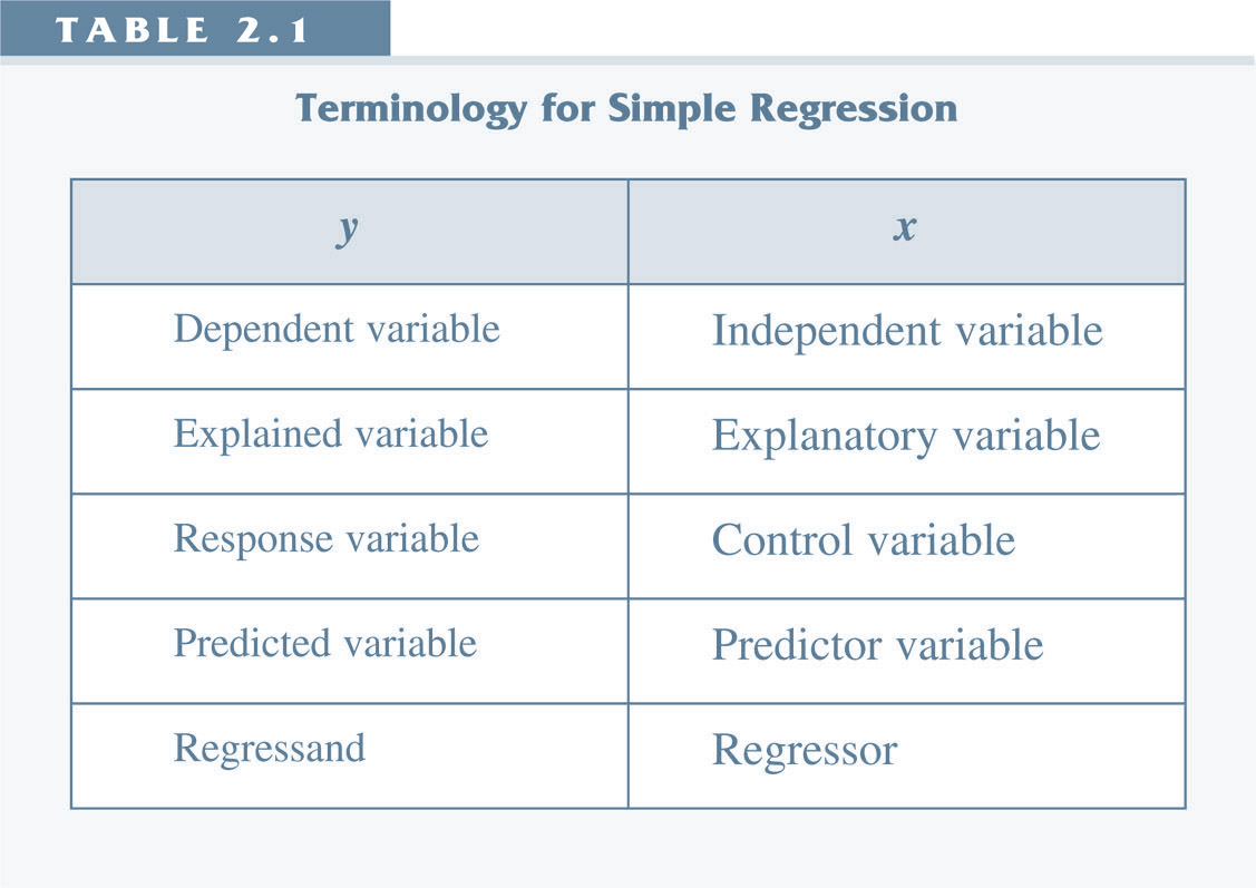
$u$: error term, disturbance term, noise.
$\beta_0$, $\beta_0$: coefficients, parameters.
$\hat{y}_i$: fitted/predicted value.
$\hat{u}_i$: residual.
$\hat{\beta}_0$, $\hat{\beta}_1$: estimators
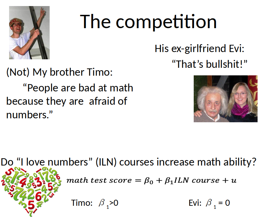
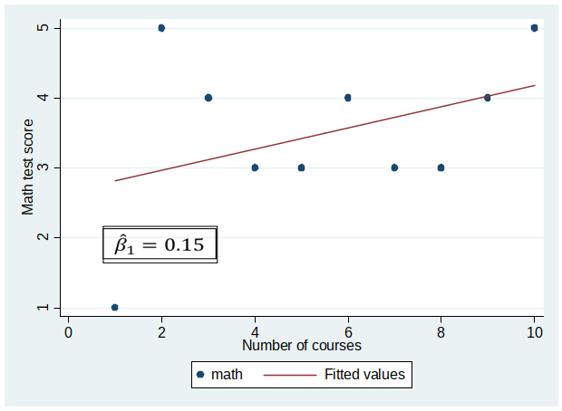
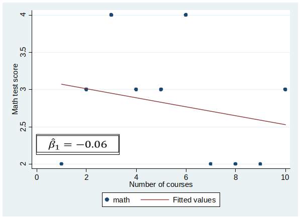
The Competition (Experiment)
- Experiment on Amazon Mechanical Turk (online labour market used by many scientists to run experiments)
- Random sample of 10 participants
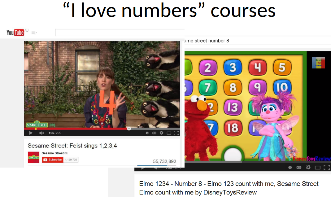
- Randomly assign people 1 to 10 “I love numbers” courses
- After this, participants take a math test, which gives scores from 1 to 5, 5 = best score.
Results of Experiment
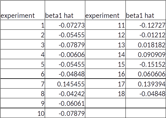
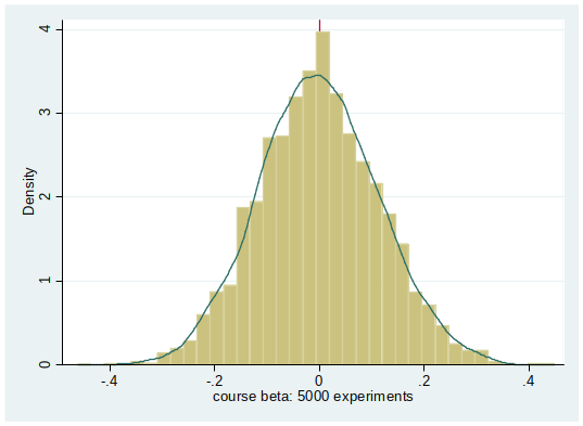
Distribution of $\hat{\beta}_1$
Disclaimer
Timo did not actually run these experiments.
I hope this story helped you to understand this very important point: $\hat{\beta}_1$ has a distribution and we only observe one realization of this distribution per sample!
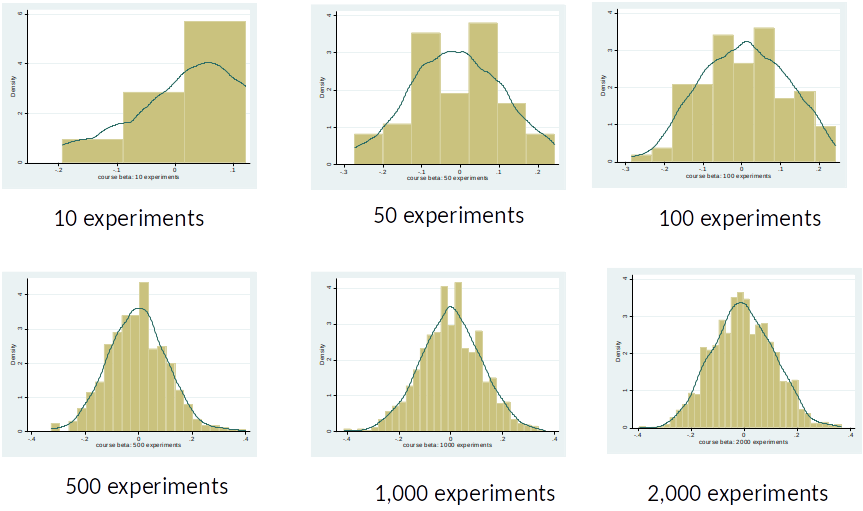
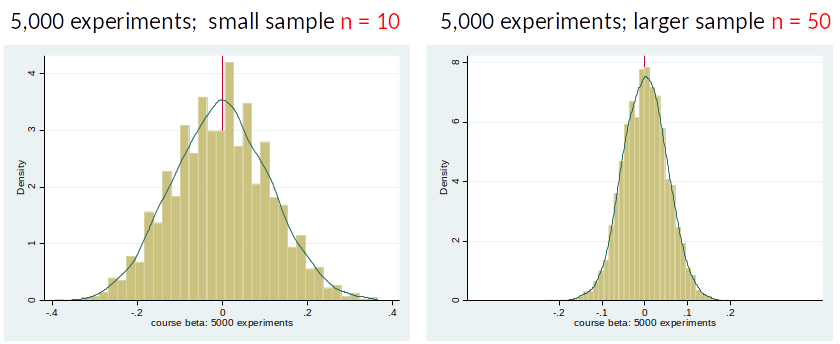
Distribution of $\hat{\beta}_1$
We assume that the parameters described in the econometric model are fixed, i.e., there is only one true $\beta_1$.
However, because we estimate our results with a (random) sample of the population, our OLS estimates will be different in each sample.
The OLS estimator $\hat{\beta}_1$ has a distribution.
We usually only have one sample and hope that our estimate is close to the true $\beta_1$.
Unbiasedness of $\hat{\beta}$
How should we evaluate whether an estimator is good?
-If $\hat{\beta}$ is equal to $\beta$? That is unlikely to happen. Not a suitable criterion.
$\hat{\beta}$ is unbiased if $E[\hat{\beta}] = \beta$
Interpretation: $\hat{\beta}$ is unbiased if the estimator is on average (in infinitely many samples) equal to the true beta.
Simple Linear Regression (SLR) Assumptions
SLR Assumptions 1-4 = conditions under which $\beta_1=\frac{Cov(x,y)}{Var(x)}$ is unbiased.
SLR 1: Linear in parameters.
(We can transform x and y, e.g., by using logs. We will talk about this later.)
Simple Linear Regression (SLR) Assumptions (cont.)
SLR 2: Random Sampling.
Our observations are taken at random from the population of interest. Random sampling ensures that the sample has, in expectations, the same characteristics as the population.
SLR 3: Variation in the Explanatory Variable.
Not all x have the same value.
Simple Linear Regression (SLR) Assumptions (cont.)
SLR 4: Zero Conditional Mean $$E[u|x] = 0$$
In practice, this is the most critical assumption.
$E[u|x] = 0 \implies E[u|x] = E[u]$ and $ $E[u]=0$.
Note: $E[u|x] = E[u]$ is sufficient for unbiasedness of $\hat{\beta}_1$, while $E[u]=0$ gives us that $\hat{\beta}_0$ is also unbiased.
$E(u|x) = E(u)$ is most plausible in a randomized experiment.
How can unbiasedness fail?
- Unbiasedness fails if any of the SLRs fail (linearity, random sampling, variation in x, zero conditional mean).
- In practice, the SLR.4 is the most important one.
- The possibility that $x$ is correlated with $u$ is very often a concern in simple regression analysis.
Variance of OLS estimator
We know now that under SLR 1-4, the OLS estimator is unbiased.
We also want to know how far away $\hat{\beta}$ is from $\beta$?
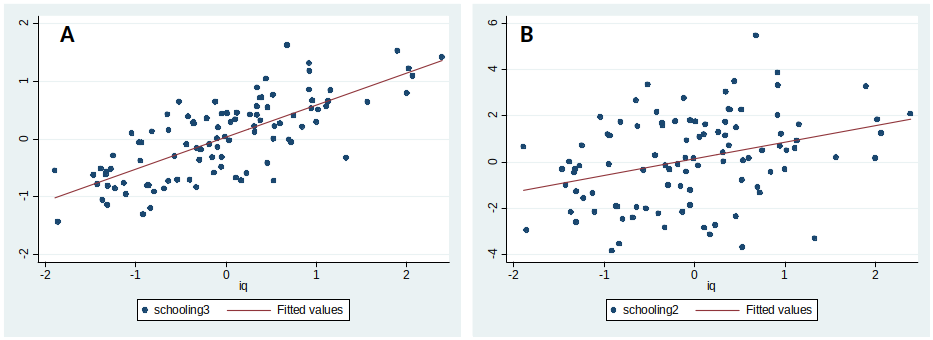
Variance of OLS estimator (cont.)
Consider the following distributions of $\hat{\beta}$
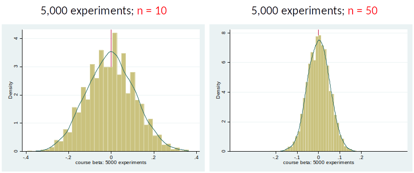
We prefer an estimator with a smaller variance.
Variance of OLS estimator (cont.)
We need an additional assumption to estimate the variance of $\hat{\beta}$ (And we need the variance to make inference about $\beta$, see topic 4).
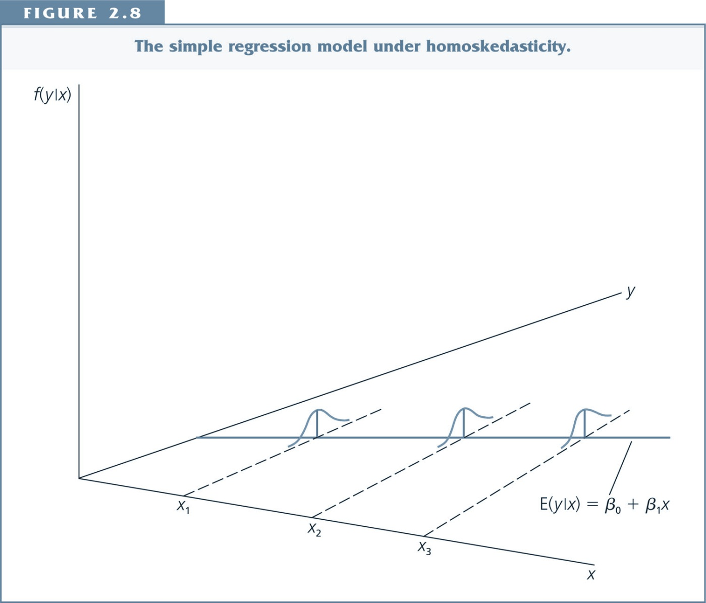
SLR 5: $Homoskedasticity$
The error term $u$ has the same variance given any value of $x$. Formally: $Var(u|x) = \sigma^2$
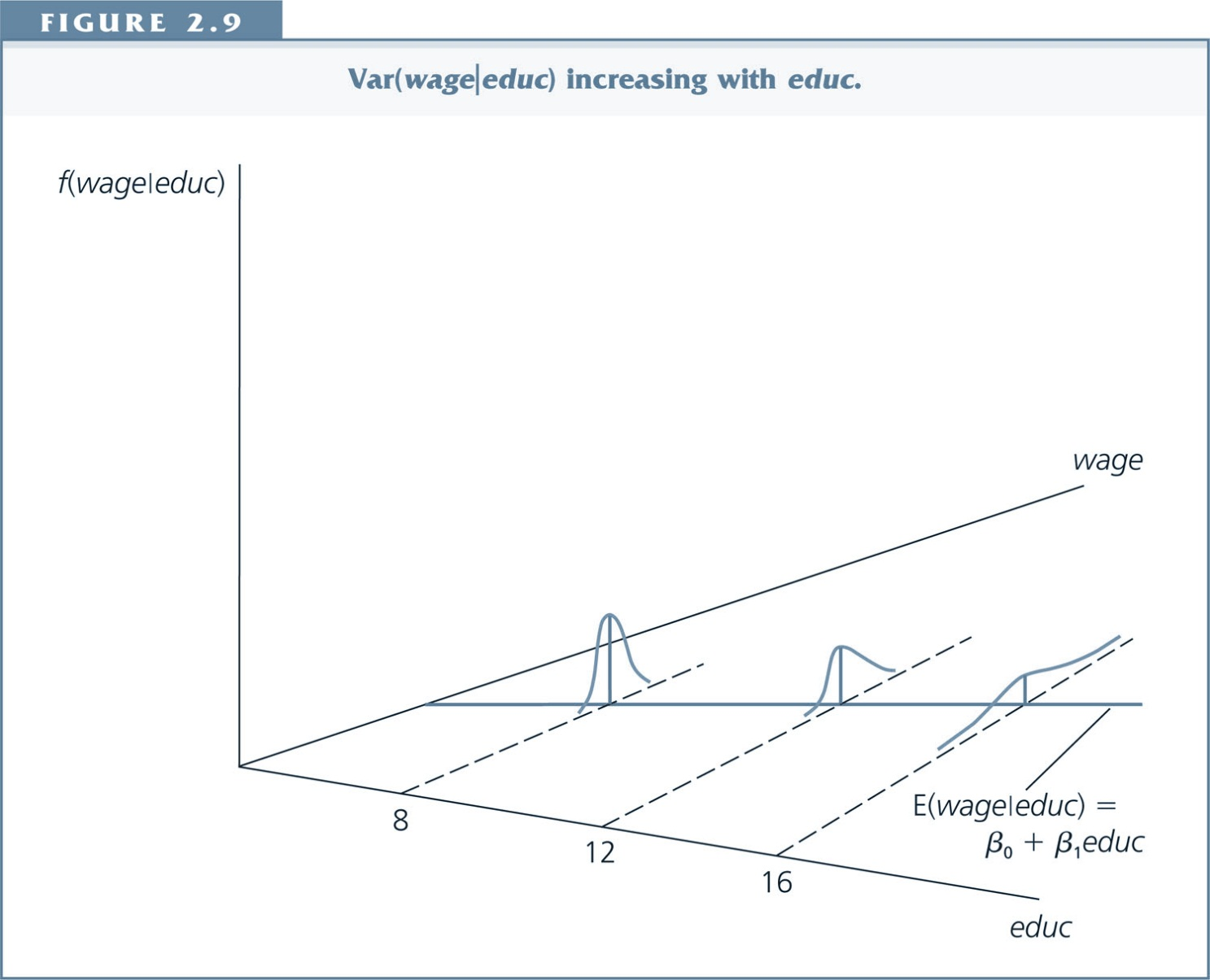
If the variance of $u$ depends on $x$, the error term is said to exhibit heteroskedasticity.
Note: $\sigma^2$, the Population Variance of $u$ equals $\frac{\sum^{N}_{i=1} (u_i-\mu_u)^2}{N}$ (note also that if our earlier assumptions hold then $\mu_u=0$)
Homoskedasticity
Heteroskedasticity
Sampling variance of the OLS estimator
Under assumptions SLR.1 through SLR.5, $$ Var(\hat{\beta}_1) = \frac{\sigma^2}{\sum^n_{i=1}(x_i-\bar{x})^2}$$
(We refer to the denominator $\sum^n_{i=1}(x_i-\bar{x})^2$ as $SST_x$, the 'sum of squares total of x')
You can see that $Var(\hat{\beta}_1)$ decreases when,
- error variance, $\sigma^2$, is low.
- we have a large sample.
- there is a high variability of $x$.
Estimator of variance of $\hat{\beta}$
Estimator for $\sigma^2$: $\hat{\sigma}^2=\frac{SSR}{n-2}$
Estimator for $Var(\hat{\beta}_1)$:
$$\widehat{Var}(\hat{\beta}_1)=\frac{\hat{\sigma}^2}{\sum^n_{i=1}(x_i-\bar{x})^2}$$
Even though we only have one sample and one realisation of $\hat{\beta}_1$, we can get an estimate of variance of the distribution of $\hat{\beta}_1$!
Can rewrite: $\widehat{Var}(\hat{\beta}_1)=\frac{SSR}{(n-2)*SST_x}$, $SSR$ is called 'sum of squares residual' and is $SSR=\sum_{i=1}^n \hat{u}_i^2=\sum_{i=1}^n (y_i-\hat{y}_i)^2$.
Preview Inference
When can we conclude that $\hat{\beta}_1 \neq 0$?
If $\hat{\beta}_1$ is large in absolute terms (far away from zero) and variance of $\hat{\beta}_1$ is small. (We will talk more about this in topic 4)
[E.g., in left figure it seems that the true $\beta_1$ might be -2, but in the right figure this seems unlikely.]
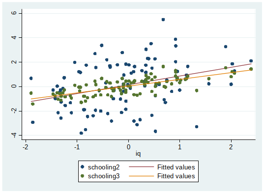
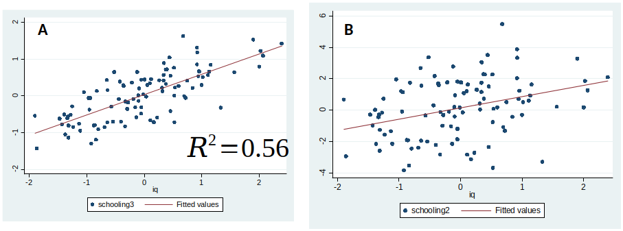
What is the difference between these two graphs?
What is the difference?
Goodness of Fit
It is often interesting to know how well the regression line fits the data.
What would be a starting point for a Goodness of Fit measure?
Better Fit = observation closer to regression line $\to$ smaller residuals.
Towards a goodness of fit measure
For each observation $i$, write $$ y_i=\hat{y}_i + \hat{u}_i $$
We can view OLS as decomposing $y_i$ into two parts:
- A fitted value
- And a residual
where the fitted values and residuals are uncorrelated in the sample.
SST, SSE and SSR
$SST$ = Total Sum of Squares
This is simply the total sample variation in $y_i$:
$$ SST= \sum^n_{i=1} (y_i-\bar{y})^2 $$
Divide $SST$ by $n-1$ $\to$ estimator of variance of $y_i$.
(a.k.a sum of squares total)
SST, SSE and SSR
$SSE$ = Explained Sum of Squares
This is the sample variation in fitted/predicted values $\hat{y}_i$:
$$ SSE= \sum^n_{i=1} (\hat{y}_i-\bar{y})^2 $$
$SSR$ = Residual Sum of Squares
This is the sample variation in the OLS residual $\hat{u}_i$:
$$ SSR= \sum^n_{i=1} \hat{u}_i^2 = \sum^n_{i=1} (y_i-\hat{y}_i)^2 $$
We can show that $$ SST=SSE + SSR $$
SST, SSE, SSR in the Stata regression output
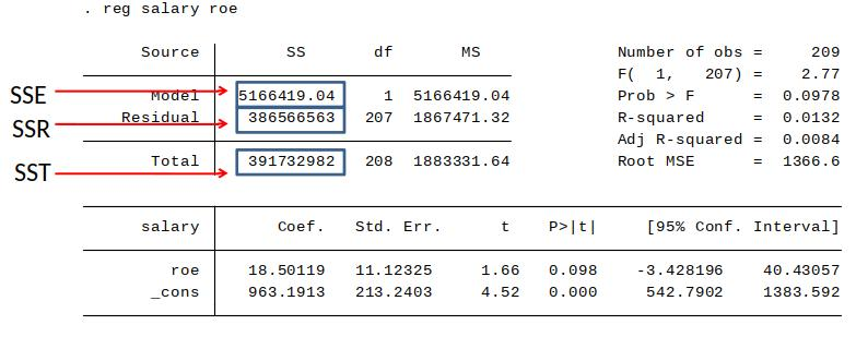
These quantities can be used to calculate a measure of the goodness-of-fit of our model.
SST, SSE, SSR in the Stata regression output
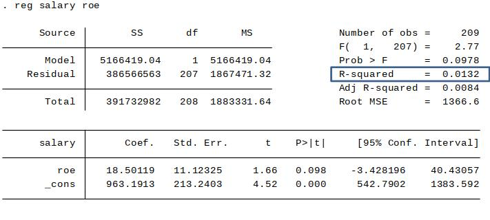
This is the $R^2$ ('R-squared') of the regression. (Sometimes called the coefficient of determination.)
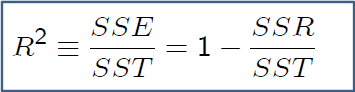
How to interpret the $R^2$?
$$ R^2 = \frac{SSE}{SST} = 1- \frac{SSR}{SST}$$
Answer: The fraction of the sample variation in $y$ that is explained by the model (here $x$).
$R^2$ is always between 0 and 1.
Additional points on $R^2$
Low R-squareds in regressions are not uncommon. In particular, if we are working with noisy cross-sectional micro data, we often get a low $R^2$.
In time series econometrics, we often get high $R^2$. Even simple models like $y(t) = a + b*y(t-1) + u$ tend to give high $R^2$.
For pure forecasting models, having a good fit (high $R^2$) is of course very central/important.
- But maximising the $R^2$ is not a goal in most empirical studies. (The focus is often instead about causation.)
- ”Students who are first learning econometrics tend to put too much weight on the size of the R-squared in evaluating regression equations” (Wooldridge, p.41).
Review/Other
Review: Distribution of $\hat{\beta}$
The OLS estimator $\hat{\beta}$ has a distribution.
The estimator is unbiased if it is correct on average (across infinitely many samples).