Intro: What is econometrics?
Causation?
Differences in Means
Randomized Experiments
Reference: Angrist and Pischke, Chapter 1.
What is econometrics?
Econometrics is a set of statistical tools that allow us to learn about the world using data.
Difference from most Statistics and Machine Learning?
Economists/Econometricians put much greater emphasis on causation.
The relationship between X and Y
We usually want to know how one particular factor (X) influences one particular outcome (Y).
What is the causal relationship between X and Y? For example, we could ask about the causal relationship between:
- Health insurance and health?
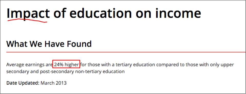
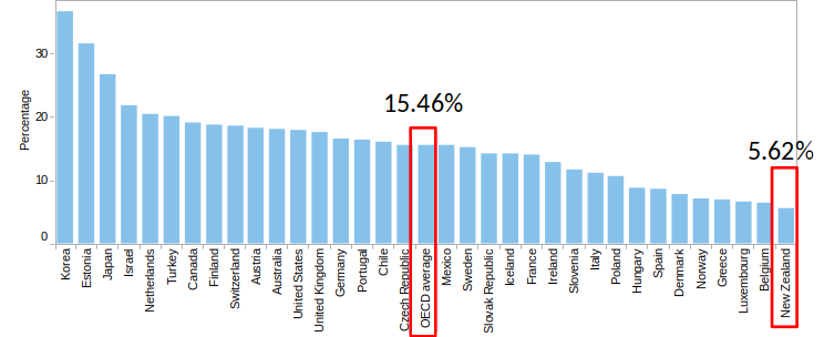
- Education and wages?
- Class size and student test scores?
- Unemployment rate and crime?
Economics: Stories and Patterns.
Theories are the stories. Data are the patterns.
We want to understand which of our stories about how the world works fit the patterns we see in the world.
We also use the data to measure the size/importance of different effects/theories.
What is the causal effect of health insurance on health?
Outcome (Y): Answer to question: Would you say your health in general is excellent (5), very good (4), good (3), fair (2), poor (1).
Treatment (X): having health insurance.
Treatment group: people with insurance.
Comparison or control group: people without insurance.
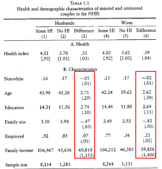
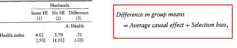
What is the causal effect of health insurance (X) on health (Y)?
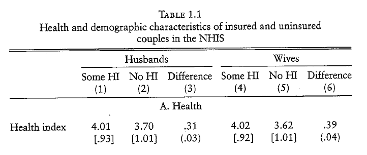
- People with health insurance (Some HI) are more healthy than people without insurance (No HI).
- Does this mean having health insurance causes better health?
ceteris paribus: other things equal
To be able to infer causality, the ceteris paribus condition needs to hold. Ceteris paribus is latin for other things equal.
Video: mru.org/courses/mastering-econometrics/ceteris-paribus
Causal effect
Causal effect for a specific individual: Health with insurance – health without insurance
$$Y_{1i} - Y_{0i}$$
1 or 0 indicate treatment:
- 1 = with health insurance
- 0 = without health insurance
i states that it is a specific individual:
- $Y_{1,Khuzdar}-Y_{0,Khuzdar}$
- $Y_{1,Maria}-Y_{0,Maria}$
People either have insurance or they don’t. We only observe one potential outcome.
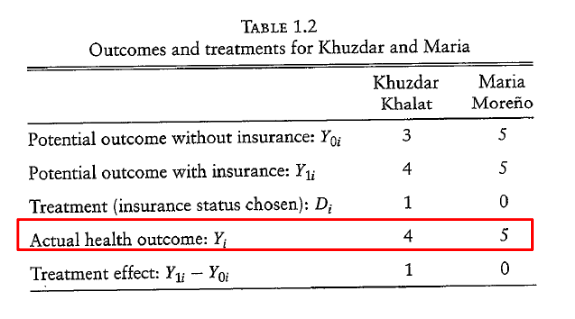
What is the causal effect of health insurance for Khuzdar and Maria?
What is the difference between actual health between Khuzdar and Maria?
$$Y_{Khuzdar} - Y_{Maria}=-1$$
What is driving the actual differences in health?
Difference because of the treatment and difference because of other factors.
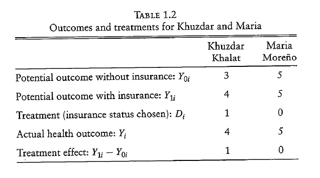
$$ \begin{align} Y_{Khuzdar}-Y_{Maria} &= Y_{Khuzdar,1}-Y_{Maria,0} \\ &= \underbrace{Y_{Khuzdar,1}-Y_{Khuzdar,0}}+\underbrace{Y_{Khuzdar,0}-Y_{Maria,0}} \\ &\quad \text{Treatment Effect} \quad + \quad \text{Selection Bias} \end{align} $$
$$ \begin{align} \text{Difference in Group Means }&=\text{ Average Y of Treated }-\text{ Average Y of Control} \\ &= Avg_n[Y_i | D_i=1] - Avg_n[Y_i | D_i=0] \\ &= Avg_n[Y_{1,i} | D_i=1] - Avg_n[Y_{0,i} | D_i=0] \\ &= (Avg_n[Y_{0,i} | D_i=1] + \kappa) - Avg_n[Y_{0,i} | D_i=0] \\ &= \kappa + (Avg_n[Y_{0,i} | D_i=1] - Avg_n[Y_{0,i} | D_i=0]) \\ &= \text{(Average) Causal Effect} + \text{Selection Bias} \end{align}$$
This is just the same as we said earlier, but with equations. And averages!
1st-to-2nd line: Definitions.
2nd-to-3rd line: Follows from treatment/control.
3rd-to-4th line: Constant effects assumption: $Y_{1,i}=Y_{0,i}+\kappa$.
4th-to-5th line: Just changes grouping of terms.
5th-to-6th line: Definitions.
$$ D_i = \left\{ \begin{align} & 1 \text{ if } i \text{ is insured} \\ & 0 \text{ otherwise} \end{align} \right. $$
Making sense of mean differences
What is the likely sign of the selection bias?
- If people with insurance are healthier in the absence of insurance = positive selection.
- If people with insurance are unhealthier in the absence of insurance = negative selection.
0.31 = Average causal effect + positive number
Average causal effect = 0.31 – positive number
We expect the average causal effect of health insurance to be smaller than 0.31.
0.31 is an upper bound on the effect of health insurance on health.
Summary so Far.
- We are interested in causal effects.
- Difference in Group Means = Average Causal Effect + Selection Bias
- These Group Means can still tell us about upper (or lower) bounds on the size of the causal effect (if we know direction of selection bias).
(made up) mean differences
People who wear a tie earn on average 20% more. Should you wear a tie to work?
People who are in a hospital have a 200% greater likelihood of dying in the next year.
Children who have books at home are 10% more likely to go to university.
Gender Wage Gap
- Gender wage gap = difference between male and female median wages, divided by male median wage.
Is this an upper bound or lower bound on gender discrimination in wages?
Making sense of mean differences
The likely direction of selection bias allows us to say if mean differences are an upper or lower bound of the average causal effect.
- Positive selection = mean differences are an upper bound
- Negative selection = mean differences are a lower bound
However, in many cases the direction of the selection bias is not clear.
We are also interested in the size of the effect.
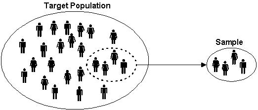
Important statistical concepts: Population and Sample
- A population is a complete set of items that is the subject of a statistical analysis.
- Example: New Zealand citizens.
- A sample is a subset of items drawn from the population.
- Example: random sample of New Zealand citizens
In econometrics, we typically want to learn about the population by looking at a sample.
Population and Sample
- In econometrics we typically prefer to have a random sample of the population, because random samples are plausibly similar to the population.
Expected Value
The expected value of $Y$, denoted $E[Y]$, is the population average of the variable $Y$.

Example: If $Y$ is the age of New Zealand citizens, then $E[Y]$ is the average age of New Zealand citizens.
Conditional expectation
The conditionally expected value of $Y$ given $x$ occurred, denoted $E[Y|X=x]$, is the population average of the variable $Y$ after conditioning on $x$ occurring.
Example: If $Y$ is the age of New Zealand citizens, and $X$ is cities in New Zealand, and $x$ is Wellington, then $E[Y|X=x]$ is the average age of New Zealand citizens living in Wellington.
If $Y$ is generated by a random process, such as rolling a dice... ($Y$ is the number rolled)
The Expected Value, $E[Y]$, is the average value of infinitely many rolls.
If $X$ is family members and $x$ is mother, then the Conditional Expectation, $E[Y|X=x]$ is the average value of infinitely many rolls by mother.
Question for the class:
What can we say about the age difference between students who are randomly chosen to sit in the front or back in a lecture hall?
Compared to students sitting in the back, students sitting in the front…
A) are on average younger
B) are on average the same age
C) have the same expected age
D) it is not possible to tell
Randomized experiments
- Randomized experiments are considered the gold standard in econometrics.
- Evidence from experiments is considered the most credible method for establishing causation.
The Reason:
- Random assignment offers a way to eliminate selection bias and to make ceteris paribus comparisons.
Intuition: If a treatment is randomly assigned, treatment and control group are comparable so that we can attribute the difference in outcome to the causal effect of the treatment.
Random assignment eliminates selection bias
$D$ is treatment status ($D = 1$ if insurance, $D = 0$ if no insurance).
If D is randomly assigned, treatment and control group will be in expectations equally healthy in absence of insurance.
Formally: $E[Y_0 | D=1] = E[Y_0|D=0]$
The difference between treatment and control group can in expectations therefore be attributed to the average causal effect (ACE) of the treatment.
Formally, with randomization: $E[Y_1 | D=1] - E[Y_0|D=0]$ = Average Causal Effect
(Reminder: Selection Bias = $E[Y_0 | D=1] - E[Y_0|D=0]$. So equals zero.)
(Notice: Expectations, so this is about the population, not the sample.)
Law of Large Numbers
The Law of Large Numbers (LLN) states that as the sample gets larger, the sample average becomes closer to the expected value.
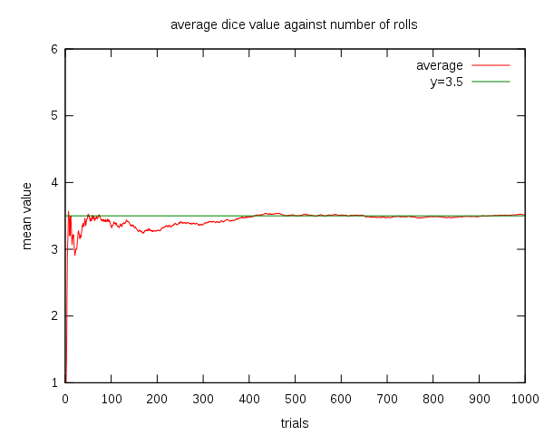
$Avg_n[Y] \to E[Y]$ as $n$ goes to infinity.
Random assignment eliminates selection bias
This is in expectation. In any sample treatment and control group might differ by chance.
However, due to the LLN the difference in health in the absence of health insurance will be small if the sample is large.
If the sample is large, the mean difference in outcomes between the treatment and control group give us a good estimate of the average causal effect of the treatment.
The Oregon health experiment
- Elegible people could register on a waiting list for health insurance.
- Out of those on the waiting list, 29,835 were randomly chosen and given the opportunity to apply for free health insurance.
- About 30% of the lottery winners (those given the opportunity) actually applied and met the criteria to receive free health insurance.
Treatment group = lottery winners
Control group = lottery loosers
Outcomes: Various health measures.
Checking for balance
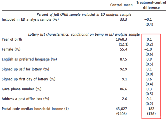
As we would expect under random assignment: there are only very small differences between treatment and control group.
Question for Class
If we can check for balance. Why do we need randomization? Why not just explictly allocat people so that our treatment and control groups are balanced?
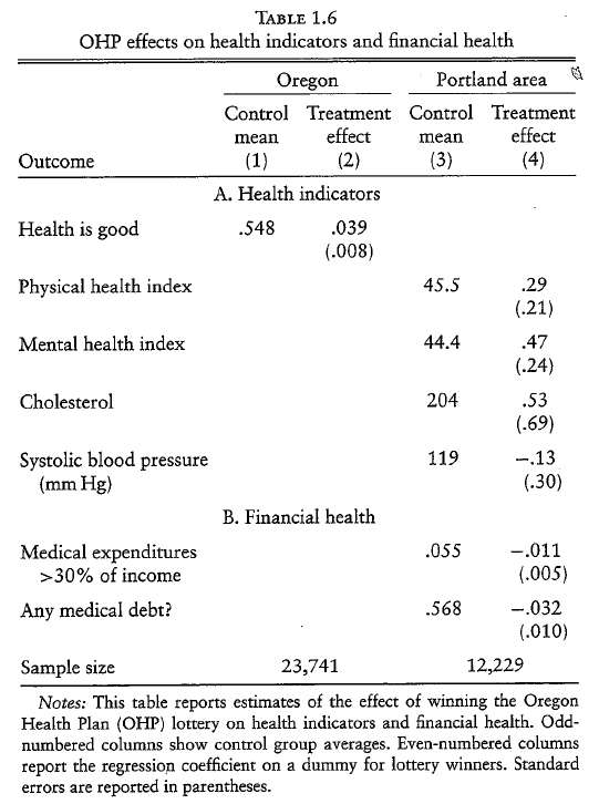
Results from Oregon Health Program
- Access to health insurance
- has a small positive effect on self-reported health and mental health.
- has a positive effect on financial situation.
- has no significant effect on physical health.
- increased emergency-department visits.
(Background knowledge: In USA, the government does not provide free medical treatment, but does provide free emergency-medical treatment. Hence the 'emergency department'.)
(Background info: Oregon gave the free coverage to everyone after a few years, the random lottery was because they could only afford to roll it out gradually due to the cost.)
Question for class (only loosely related)
Interpreting results is not always easy:
In Microeconomics, when talking about Insurance we often talk about imperfect information and how this leads to adverse selection and moral hazard.
What might adverse selection imply for these results and their interpretation?
What might moral hazard imply for these results and their interpretation?
Racial discrimination in the labor market
Black Americans earn less than White Americans in the US.
Suggests racial discrimination. But can we be certain?
Black Americans may differ from White Americans on average in ways that affect earnings, so simply looking at wage differences is not enough as evidence for discrimination.
- Is the wage difference likely an upper or lower bound?
Can we do an experiment by randomly assigning race?
Bertrand and Mullainathan (2004) sent out fake CVs in response to newspaper ads which were otherwise identical but some had Black sounding names (e.g., Jamal) and others White sounding names (e.g., Greg).
They sent out 4,870 CVs (50% black names)
Results:
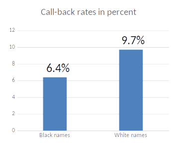
Having a black name on a CV causes a lower response rate.
Racial discrimination in the labor market
Does this translate into differences in actual job offers?
Is this evidence of taste based discrimination (i.e., a dislike of black people)?
Or is this evidence of statistical discrimination (i.e., maybe employers believe - rightly or wrongly - that applicants with black sounding names are less productive.
Replication Study (1/3)
A more recent paper could not replicate the effect.
They found almost identical call-back rates for CVs with black and white names.
Replication Study (2/3)
One key difference between the original and replication study was the names chosen.
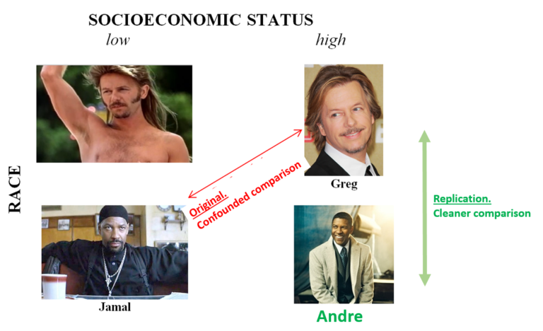
Replication Study (3/3)
The results in the original paper might have been driven by bias against low socio-economic status names.
However, it could also be driven by other factors (e.g. different study period).
Limitations of Experiments
Gold-standard, but not a Silver bullet.
- Randomized experiments are the most credible evidence of causation.
- However, they also have limitations (many of which apply to other methods as well):
- The long-term effects might be different.
- External Validity: It is not clear if results tell us something about other settings. (e.g., Do results of an experiment in Kenya tell us anything about Uganda?, about India?, about Germany?)
- People might have behaved differently because they knew that they were part of an experiment (experimental effects / Hawthorne effect).
- The effect might be different if it is implemented at a large scale (general equilibrium effects). E.g., maybe job-training helps you get a job because you are now more trained than everyone else. If we give everyone job-training then no-one is 'more trained' than the others, so effect is much smaller.
More prosaically, random experiments are often expensive. The 2019 Nobel Memorial Prize in Economic Sciences went to Banerjee & Duflo. You can read about their work with 'Randomly Controlled Trials' (field-experiments) in their book Poor Economics - A Radical Rethinking of the Way to Fight Global Poverty.