Revision
- Revision
Information about Exam
Reference: Wooldridge
What is Econometrics About?
The goal: We want to test our ideas about how the world works using data.
Econometrics is a toolbox that helps us to do this.
The relationship between X and Y
We usually want to know how one particular factor (X) influences one particular outcome (Y).
What is the causal relationship between X and Y? For example, we could ask about the causal relationship between:
- education and wages
- class size and student test scores
- smoking and health
- unemployment rate and crime
DGP and econometric model
We believe that there is some process – the data generating process (DGP) - that explains how the outcome we observe is generated.
We describe this DGP mathematically with an econometric model.
When writing down the econometric model we therefore have to think about how the functional form (exponential, quadratic, etc.) of the relationship between Y and our Xs.
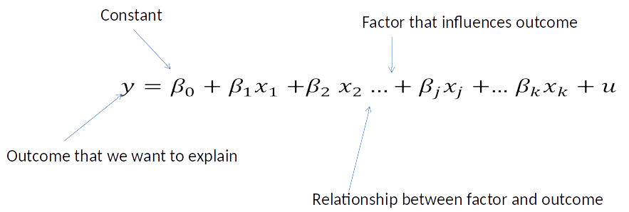
The $\beta$ Coefficient
- $\beta_j$ (or any $\beta$, $j$ is just an example) shows how change in one factor ($x_j$) affects the outcome: $$\beta_j = \frac{\text{change in }y}{\text{change in }x_j} = \frac{\Delta y}{\Delta x_j}$$ $$ \Delta y = \beta_j \Delta x_j $$
- If we would increase $x_j$ by one, holding all other factors constant, $y$ will change by $\beta_j$.
- $\beta_j$ shows the causal change of an change in $x_j$ on $y$.
Simple and Multiple Regression Model
Simple Regression model: $$ y=\beta_0 + \beta_1 x + u $$ (mention only one factor, x, explicitly)
Multiple Regression model: $$ y=\beta_0 + \beta_1 x_1 + \beta_2 x_2 + u $$ (mention more than one factor, here $x_1$ and $x_2$, explicitly)
What do we really want to do?
- Find $\beta_j$!
Why? Because $\beta_j$ describes the causal relationship between $x_j$ and $y$. This is important for good decision making.
We use data to do this. In a way Economists can also be considered Data Detectives.

How do we find $\beta_j$?
Collecting and analysing data.
The most popular method for analysing data is OLS (others are FD, IV).
In some very special circumstances (see OLS assumptions) OLS gives us good estimates of $\beta_j$.
Vocabulary guidelines
Greek letter = parameter (unobserved and unknown)
Greek letter with hat = estimator of parameter (what you see in Stata)
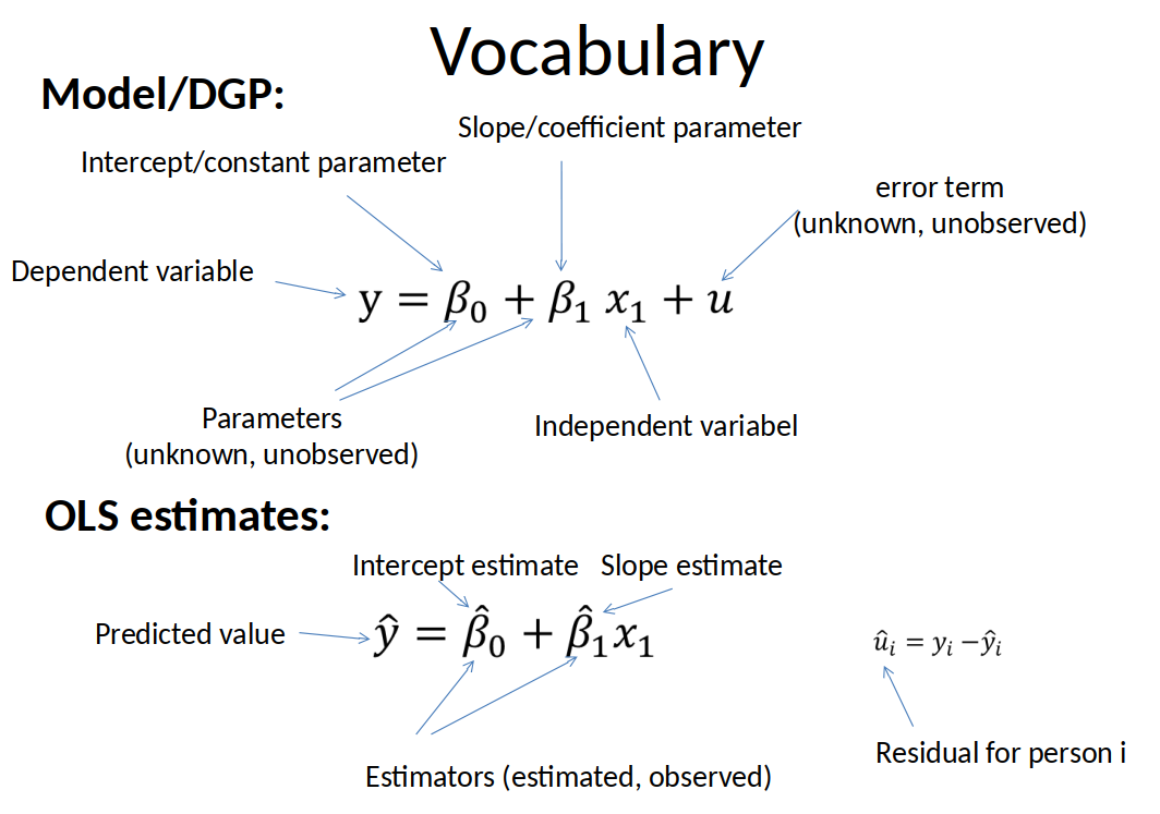
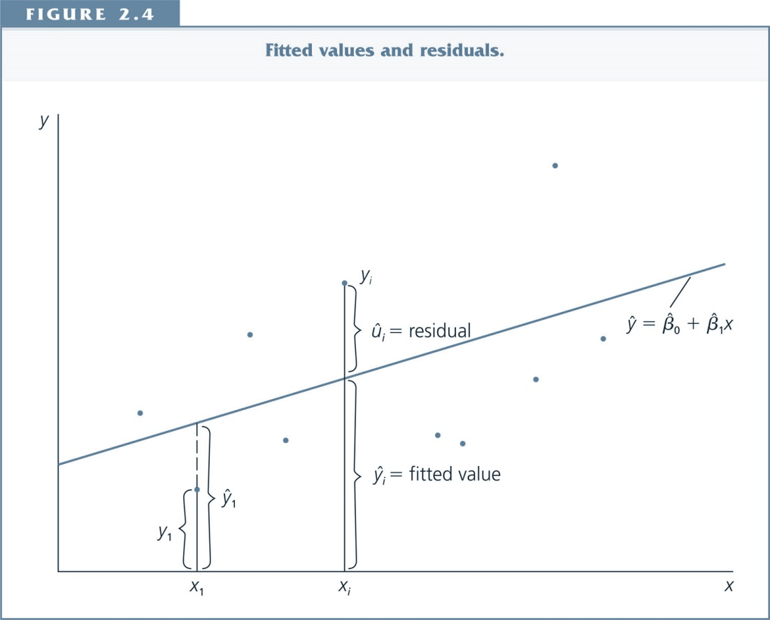
The Mechanics of OLS
- In any dataset, OLS chooses values of the estimators ($\beta_1$,$\beta_2$,...) to minimize the sum of squared residuals.
Beware! OLS does not imply causation
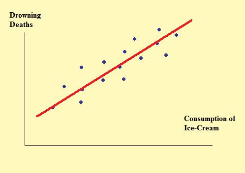
$\hat{\beta}_j$ is not the same thing as $\beta$.
Distribution of $\hat{\beta}_j$
- Our OLS estimate is done with one sample.
- For each (hypothetical) new sample we would get a different estimate.
- All the values of the hypothetical estimates follow a distribution. This is what we mean with distribution of $\hat{\beta}_j$.
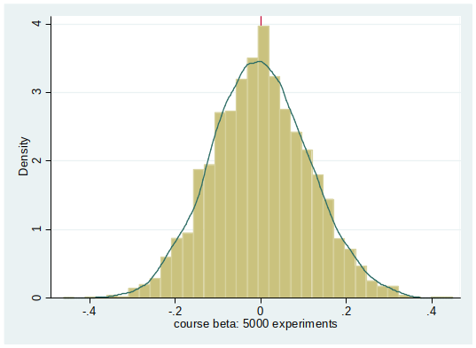
Unbiasedness of $\hat{\beta}_j$
Formal definition: $\hat{\beta}_j$ is unbiased if $E[\hat{\beta}_j] = \beta_j$.
Intuition:
- $\hat{\beta}_j$ is and unbiased estimator of $\beta_j$ if $\hat{\beta}_j$ is on average (in infinetely many samples) equal to $\beta_j$.
- Since we know that with each sample we would get a different estimate, we aim for having an estimator that gets it right on average.
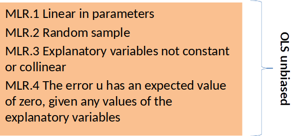
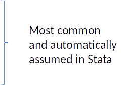
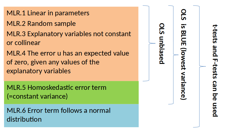
When is $\hat{\beta}_j$ unbiased?
- When Multiple Linear Regression (MLR) assumptions 1-4 are fulfilled.
Another quality criteria: consistency
An estimator is consistent if as n (the sample size) tends to infinity, the distribution of $\hat{\beta}_j$ collapses to the single point $\beta_j$.
In other words: consistency means that the estimator is correct if we have an infinetley large sample.
Under assumptions MLR.1-4, $\hat{\beta}_j$ is a consistent estimator of $\beta_j$.
Hypothesis Testing
Now we know when $\hat{\beta}_j$ is correct on average in many samples (i.e., unbiased), but we typically only have one sample.
Can we ever know the exact value of $\beta_j$? No.
But, under some circumstances we can draw conclusions about the value of $\beta_j$. For example:
- Is $\beta_j$ 0?
- In which interval can we expect $\beta_j$ to be? (Confidence Interval)
Null and alternative Hypothesis
We specify the null and alternative hypothesis. Typically:
Null hypothesis
- (H_0): $\beta_j= 0$
- Alternative hypothesis two sided
- (H_1): $\beta_j \neq 0$
- (H_1): $\beta_j \neq 0$
Note: Sometime the null hypothesis is that $\beta_j$ is equal to a particular value, and sometimes the alternative hypothesis is one sided.
Hypothesis Testing
- Under which circumstances can we draw conclusions about $\beta_j$?
- If MLR 1-6 are fulfilled.
- We have just seen MLR 1-4. Let’s have a look at MLR 5-6
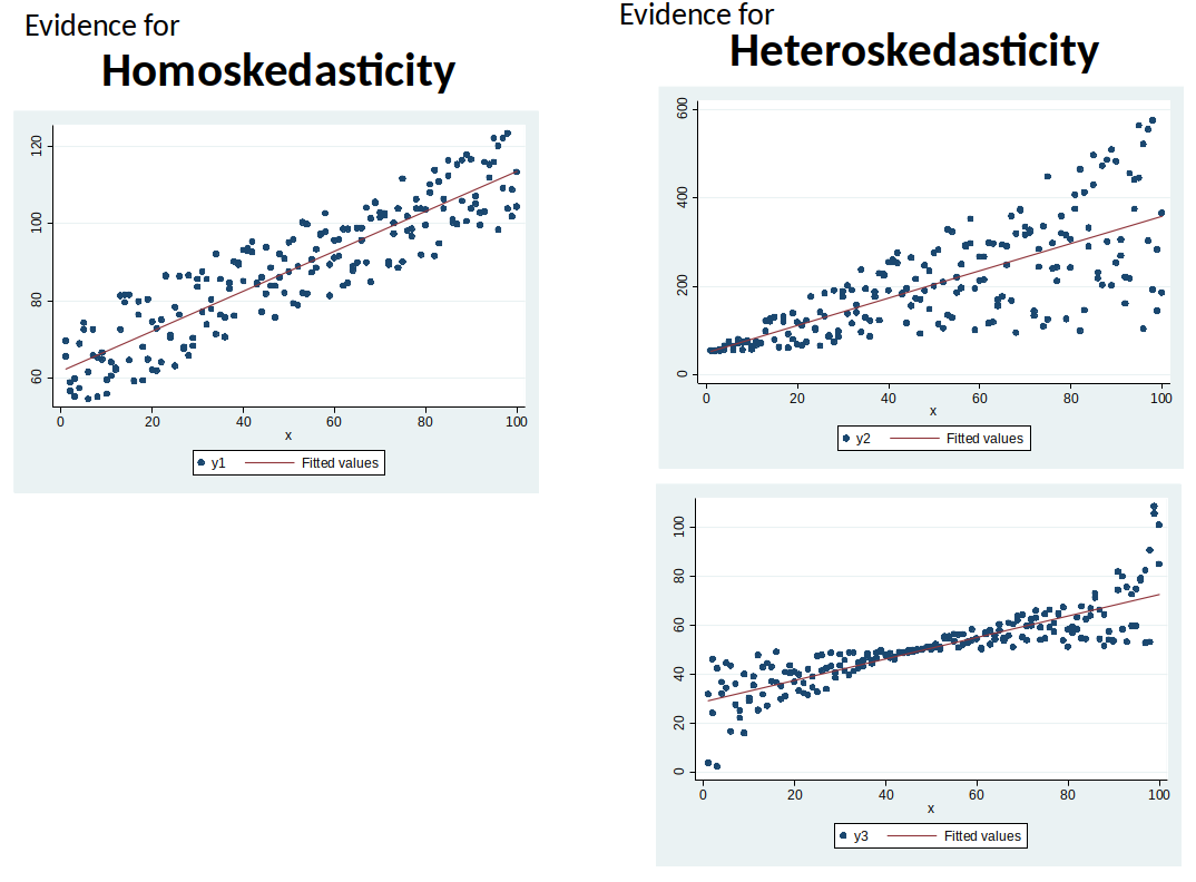
Heteroskedasticity
Assumption MLR.5: Homoskedasticity: The error u has the same variance given any value of the explanatory variables. $$Var(u│x_1, x_2,...,x_k) = \sigma^2$$
Under assumptions MLR.1-5, OLS estimator is the Best Linear Unbiased Estimator (BLUE).
(MLR.1-5 are collectively known as the Gauss-Markov assumptions)If MLR.5 is violated we have Heteroskedasticity.

Normality (MLR.6)
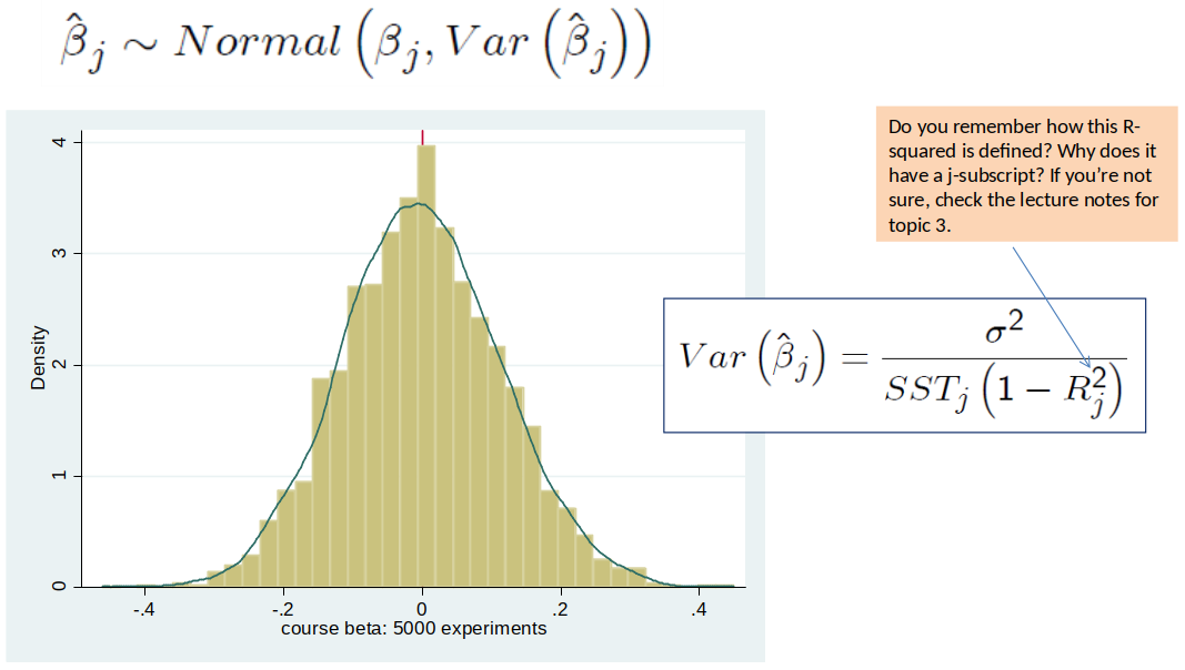
- Assumption MLR.6: Normality: The population error u is independent of the explanatory variables $x_1, x_2,...,x_k$ and is normally distributed with zero mean and variance $\sigma^2$: $u \sim Normal(0, \sigma^2)$.
Note: The Normality assumption is only necessary in small samples.
Why is normality important?
Answer: It implies that the OLS estimator $\hat{\beta}_j$ follows a normal distribution too.
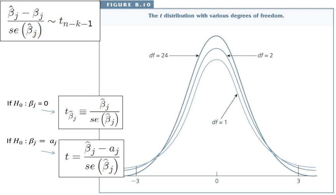
And when $\hat{\beta}_j$ is normally distributed, our t-statistic is t-distributed.
If our t-statistic is t-distributed we can know the probability of getting the t-statistic that we have if there is no effect (p-values).
If MLR 1-6 hold:
If MLR.1-6 hold:
The ratio of $\hat{\beta}_j-\beta_j$ to the standard deviation follows a standard normal distribution.
The ratio of $\hat{\beta}_j-\beta_j$ to the standard error (called t-statistic) follows a t-distribution.
The t-distribution
Hypothesis Testing, outline
t test, intuition
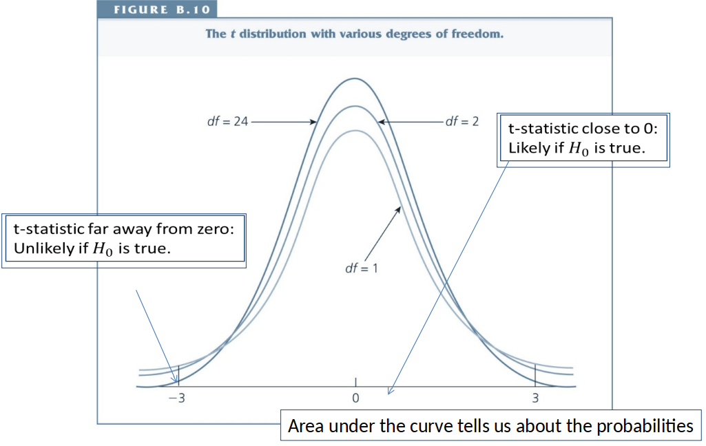
Our starting point ($H_0$) is usually to assume that the true effect is zero but our estimator is different from zero by chance.
However, if the true effect is zero, large and small t-statistics are unlikely.
When the t-statistic is large/small enough, we conclude that the true effect is probably not zero and thus reject $H_0$.
t test, intuition
When is a t-statistic large/small enough? This depends:
- Is our alternative hypothesis is one-sided or two sided (typically two sided)
- What is the probability we are willing to accept of rejecting if it is in fact true – the significance level (typically 5%)
In the past we would have looked up a critical value, c, in a statistical table and compared it to our t-statistic.
Today, Stata does this for us automatically.
Three ways of seeing if $\beta_j$ is significant
Look at p-value:
Compare p-value to significance level.
If p-value $\leq$ significance level $\Rightarrow$ reject $H_0$. If p-value $>$ significance level $\Rightarrow$ don't reject $H_0$ (Note: we never accept $H_0$)Or, use the rule of thumb for two sided alternatives:
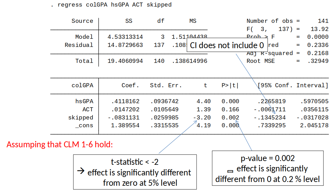
Given a 5% significance level and $df>60$, a t-value lower than -2 or higher than 2 implies statistical significance.Or check if 95 Confidence Interval includes 0.
t-statistic and p-values in Stata
A Closer look at MLR assumptions
If MLR.1-6 Holds
We can use OLS for estimation and hypothesis testing, and all is fine and dandy: OLS is then a very “good” estimator (unbiased, low variance) and it’s easy to test hypotheses.

If MLR.1-6 DO NOT hold
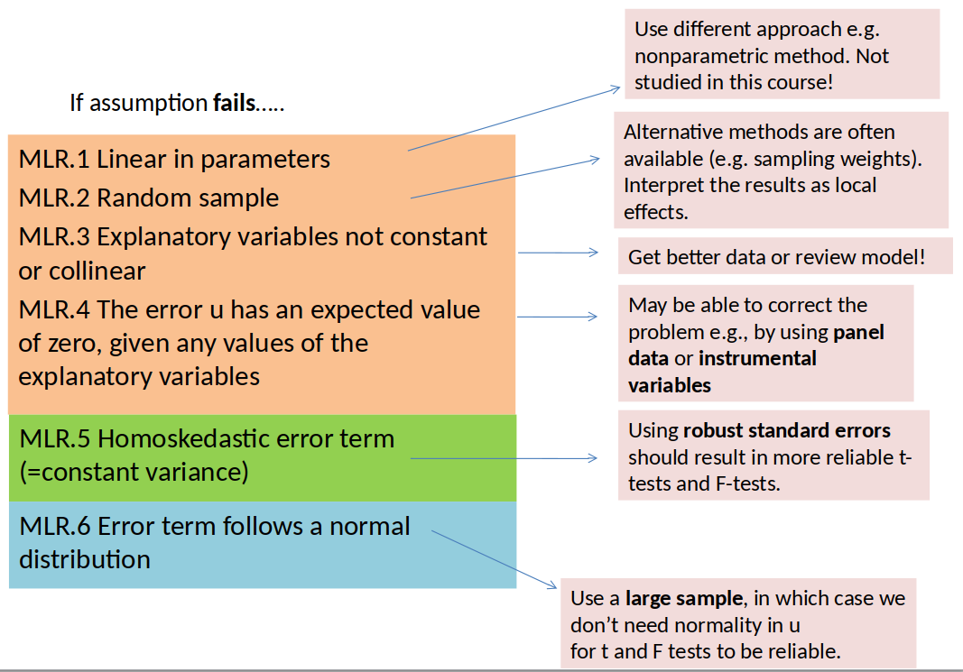
We can try to fix it.
Or we have to interpret our results differently.
Let’s have a closer look at the MLR assumptions.
If MLR.1-6 DO NOT hold
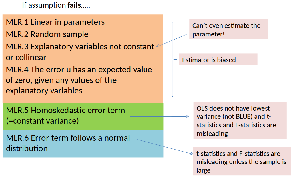
What to do if assumptions fail
What to do when your estimator is biased?
Include more relevant variables
- But, it is often difficult to collect all relevant variables
Use a different method
- Differences-in-Differences estimation
- First-Difference estimation
- Instrumental variable (IV) estimation
- These methods only work in specific circumstances --> Check their assumptions!
Difference-in-Difference (Diff-in-Diff) estimator, intuition
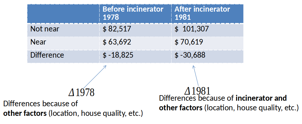
Diff-in-Diff estimator of effect of incinerator: $\Delta 1981 - \Delta 1978 = -\$11,863$
Graphical Illustration of Diff-in-Diff
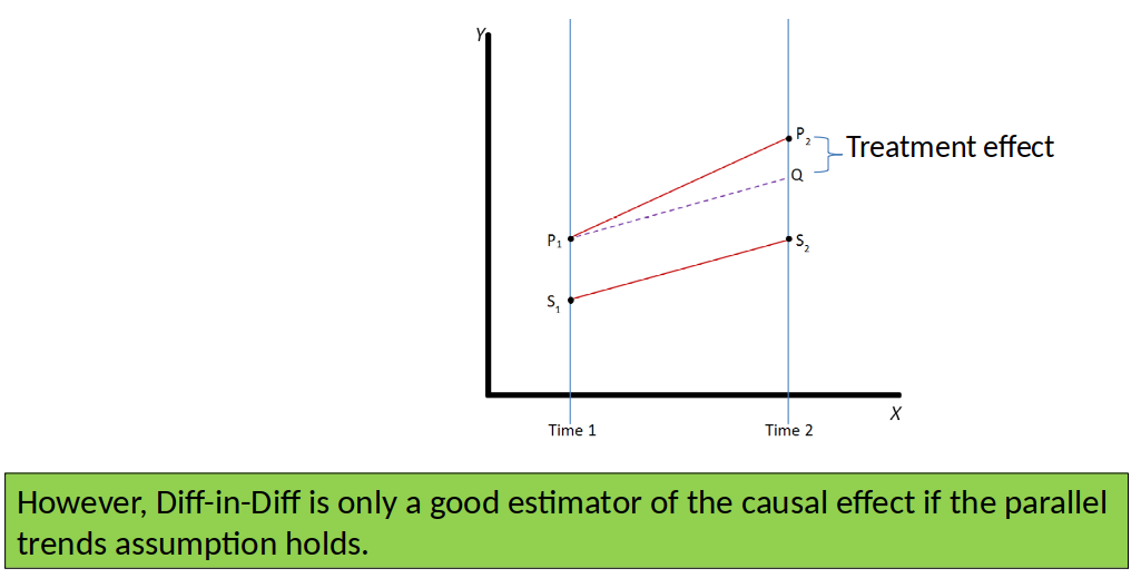
Parallel trends assumption: The outcome of the treatment and control group would have followed a parallel trend in the absence of the treatment.
First-Differences Estimaton (Fixed Effects)
Possible if we have panel data.
We relate changes in X to changes in Y.
Allows us to difference away time constant part of the error term (remember the dog and the scale).
IV estimation
Possible to get a causal effect if $x$ is endogenous.
All we need is an instrumental variable ($z$) that fulfills two assumptions:
instrument relevance: $Cov(z,x) \neq 0$
- instrument exogeneity: $Cov(z,u) = 0$
IV estimation
IV estimates are Local Average Treatment Effects (LATEs)
- average treatment effect for those who were moved by the instrument (compliers + defiers).
Monotonicity assumption:
- instrument influences the endogenous variable only in one direction
If the monotonicity assumption holds, IV estimates the average treatment effect on the treated (ATE)
Change Interpretation
Unless you have an experiment, for most research questions it is very difficult to get an unbiased estimator.
But, OLS estimates are still often very interesting even if you can’t interpret them causally.
Information about Exam
Exam Info
Final Test: 60 minutes. See precise details in Blackboard. (Specific time, focus on last parts of course.)
Final MCQ test: 50 minutes. See precise details in Blackboard. ('Any time', covers whole course.)
Topic 10 arguing with data (last lecture) will not be assessed.
- You can use a calculator.
Fill-in-the-blank questions. Numeric questions.
- For these, I look for specific numbers, terms or symbols.
Tutorial questions
These questions will be very similar or even identical to questions from tutorial exercises.
They are supposed to be easy points for students who study!
- Have a look at your tutorial exercises!
Study for Exam
- Review slides
- Review test, quizzes and assignment.
- Many questions on the exam will be very similar to questions on the test/quizzes/assignment.
- Review tutorial exercises.
- Online tests, so they are designed to be difficult to complete in the time available.
- Randomized questions. So your test will not be identical to those of other students.
Guidelines for answering exam questions
Be precise and to the point.
Avoid irrelevant and wrong explanations.
Read the instructions and questions carefully.
You might not have time to answer all questions $\Rightarrow$ Answer easy questions first.
Guidelines for answering exam questions
Try to be to the point and answer only what the questions ask. For most questions this will be a one word or one sentence answer.
Example: How many coefficients in this model (excluding the constant) are significant at the 20% level? [1 mark]
- Student answers:
Educ, exper, exper2 are all significant at the 1% level and numdep is significant at the 20% level.
All coefficients are significant at the 20% level except the nonwhite coefficient, which has a p-value that is greater than 0.2. - My answer:
4.
- Student answers:
Example of Wrong and Irrelevant Answer
Question: How many coefficients in this model (excluding the constant) are significant at the 20% level? [2 mark]
Student answer: 4, because the R-squared is 0.4
Comment: 4 is correct, but the explanation is wrong. This wrong and irrelevant addition would lead to reduction of marks.
Guidelines for answering exam questions
I will try to mark important words, but still read the questions carefully.
Example:
Exam grading/sample answers
I have a document with exam answers. [More accurately, they are built into blackboard.]
The answers on this document are very short: often one number or a few words, never longer than 2 sentences.
No marks will be given for workings.
You will be able to see what you answered, as well as correct answer, for most of the questions. But not until a day or two after all students have finished.
Questions in the next weeks? (1)
- There will be some kind of office hours support early next week. A Blackboard announcement of details will be made later this week.
Questions in the next weeks? (2)
Use the discussion board and help each other out.
I have little time next weeks, but can tune in to the discussion from time to time.
Final Words
I enjoyed this class. I hope you have learned something that you remember after the exam.
Special thanks to those who turned up in person. Made teaching much nicer for me.
Any (positive or negative) feedback on the course? Great! Talk to me or send me an email.
Good luck with the exam!