Contents

% Example based on Aiyagari (1994) that shows how to have two 'permanent types' of agents.
%
% Before looking at this you should be familiar with how to solve the model
% of Aiyagari (1994). In this example I extend the model to allow for two
% types of agents who have different discount factors: the parameter beta (they could in
% principle differ in just about anything).
% This is the second (v2) of two examples that do this. In this example the
% different types of agents are set up by giving them 'names' and making the
% parameter beta take different values for the different names (by making beta
% what matlab calls a 'structure' instead of just a scalar number).
% In the first (v1) example the exact same model was solved but instead the
% different types of agents were set up as a vector for the discount factor
% parameter beta.
%
% Essentially three changes have to be introduced to the setup: Names_i,
% which gives the names of the permanent types to be used. The change to the
% actual parameter values for beta. The 'weight' or 'fraction' of agents of
% each type (below called PTypeWeights, and PTypeDistNames).
%
% A quick comment on v1 (vector) versus v2 (names) approaches. While both
% can in principle do exactly the same thing, if you have lots of different
% types of agents, who differ in just one or two respects (e.g., ten types or one
% hundred types, but only difference is their risk aversion parameter and their
% Frisch elasticity of labour supply) then you will want to use the v1
% (vector) approach. If you have just a small number of agent types, but
% they are genuinely different (e.g., one is a finite lived household and
% the other an infinitely lived firm, or three household types representing
% single males, single females, and married couples) then you will want to
% use the v2 (structure) approach.
%
% As will be seen, other than having to be explicit about the changes when
% setting up solving a model with multiple 'permanent types' of agents using the VFI
% Toolkit is no more difficult that the model with just one type.
% It is worth mentioning that 'permanent types' is not the same thing as
% the standard econometrics concepts of 'permanent shocks' (as in unit root
% models in time series) and it is not the same thing as fixed effects in
% panel data econometrics (although you might think of it as a more
% sophisticated version of this; agents differ in a permanent way, but with
% fixed effects that must play out exactly the same every time period,
% while here 'permanent types' can play out in ways that lead to behaviour
% that in reduced form will appear to change over time.
%
% Other than allowing for two different 'permanent types' of agents this
% code does exactly the same as the standard example code for the Aiyagari
% (1994) model: https://github.com/vfitoolkit/VFItoolkit-matlab-examples/tree/master/HeterogeneousAgentModels
% That is, these codes set up and solve the Aiyagari (1994) model for a given
% parametrization. After solving the model they then show how some of the
% vfitoolkit commands to easily calculate things like the Gini coefficient
% for income, and how to plot the distribution of asset holdings.

Different permanent types of agents

Names_i={'impatient', 'patient'}; % There are two permanent types of agents.
% The other thing we will need to do is specify the different values of the parameter beta below.
% Other than this the only notable changes are that this information needs
% to be passed as an additional input to a number of the VFI Toolkit commands.
% Note: You just pass Names_i as an input in exact same way you would pass
% N_i in the v1 (vector) approach to permanent types of agents. The VFI
% Toolkit automatically recognises which of the two you are using based on
% contents of N_i or Names_i.

Grid sizes, have declared at beginning for convenience.

n_k=2^9;
n_l=21;
n_r=0; % Normally you will want n_p=0, setting a non-zero value here activates the use of a grid on prices.

Declare the model parameters (keep them all in a structure Params)

% Our two permanent types of agents differ in their values of beta. In v2
% of this we set this up using a structure for beta. Nice thing is you can
% just refer to agents by their names.
Params.beta.impatient=0.94; % Discount factor for 'impatient' type of agent.
Params.beta.patient=0.98; % Discount factor for 'patient' type of agent.

Params.alpha=0.36; % Capital share in Cobb-Douglas Production function
Params.delta=0.08; % Depreciation rate of capital
Params.mu=3; % CRRA parameter in utility function
Params.rho=0.6; % Autocorrelation of z
Params.sigma=0.2; % Std dev. of shocks to z

%Set initial value for interest rates (Aiyagari proves that with idiosyncratic
%uncertainty, the eqm interest rate is limited above by it's steady state value
%without idiosyncratic uncertainty, that is that r<r_ss).
Params.r=0.02;

Params.q=3; %Footnote 33 of Aiyagari(1993WP, pg 25) implicitly says that he uses q=3

Set up the exogenous shock process

Create markov process for the exogenous labour productivity, l.

[l_grid, pi_l]=TauchenMethod(0,(Params.sigma^2)*(1-Params.rho^2),Params.rho,n_l,Params.q);
l_grid=exp(l_grid);
% % Get some info on the markov process
[Expectation_l,~,~,~]=MarkovChainMoments(l_grid,pi_l); %Since z is exogenous, this will be it's eqm value
l_grid=l_grid./Expectation_l;

Grids

% In the absence of idiosyncratic risk, the steady state equilibrium is given by
r_ss=1/Params.beta.patient-1;
K_ss=((r_ss+Params.delta)/Params.alpha)^(1/(Params.alpha-1)); %The steady state capital in the absence of aggregate uncertainty.
Params.kmax=15*K_ss;

% Set grid for asset holdings
k_grid=exp(linspace(0,log(Params.kmax+1),n_k))'-1;
% nk1=floor(n_k/3); nk2=floor(n_k/3); nk3=n_k-nk1-nk2;
% k_grid=sort([linspace(0,K_ss,nk1),linspace(K_ss+0.0001,3*K_ss,nk2),linspace(3*K_ss+0.0001,15*K_ss,nk3)]');

% Bring model into the notational conventions used by the toolkit
% To simplify this example I have used the (a,z) notation of the VFI
% Toolkit directly.
n_d=0;
d_grid=0; %There is no d variable
n_a=n_k;
a_grid=k_grid;
n_z=n_l;
z_grid=l_grid;
pi_z=pi_l;
n_p=n_r;

Solving the value function problem

DiscountFactorParamNames={'beta'};

ReturnFn=@(aprime_val, a_val, z_val,alpha,delta,mu,r) Aiyagari1994_ReturnFn(aprime_val, a_val, z_val,alpha,delta,mu,r);
ReturnFnParamNames={'alpha','delta','mu','r'}; %It is important that these are in same order as they appear in 'Aiyagari1994_ReturnFn'

% Following lines are used to test that we are setting things up correctly, but is not needed at this stage.
vfoptions.verbose=1;
disp('Test ValueFnIter')
tic;
[V, Policy]=ValueFnIter_PType(n_d,n_a,n_z,[],Names_i,d_grid, a_grid, z_grid, pi_z, [], [], ReturnFn, Params, DiscountFactorParamNames, ReturnFnParamNames, [], vfoptions); % The unused inputs related to the possibility that some agents are what VFI Toolkit calls 'Case2' (following nomenclature of SLP1989)
toc

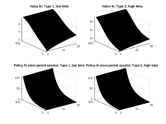
% Graph the two different value functions and the two different policy functions.
% Note that these are the example/test ones, not the ones in equilibrium.
figure(1)
subplot(2,2,1); surf(V.impatient) % NOTE: notice that relative to v1, this is now 'by name' rather than the generic pt1 and pt2
title('Value fn: Type 1, low beta')
subplot(2,2,2); surf(V.patient)
title('Value fn: Type 2, high beta')
subplot(2,2,3); surf(a_grid(shiftdim(Policy.impatient,1)))
title('Policy fn (next period assets): Type 1, low beta')
subplot(2,2,4); surf(a_grid(shiftdim(Policy.patient,1)))
title('Policy fn (next period assets): Type 2, high beta')

Solving for the stationary distribution

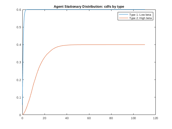
Params.PTypeWeights=[0.6; 0.4]; % Make 60% of agents the 'low beta' type and 40% the 'high beta' type.
PTypeDistNames={'PTypeWeights'};

% Following lines are used to test that we are setting things up correctly, but is not needed at this stage.
simoptions=struct();
disp('Test StationaryDist')
tic;
StationaryDist=StationaryDist_PType([],[],Policy,n_d,n_a,n_z,[],Names_i,d_grid, a_grid, z_grid,pi_z,[],[],Params,[],PTypeDistNames,simoptions);
toc

% Graph the cumulative distribution function over asset holdings.
% Note that these are the example/test ones, not the ones in equilibrium.
figure(2)
plot(a_grid,cumsum(sum(StationaryDist.impatient,2))*StationaryDist.ptweights(1))
hold on
plot(a_grid,cumsum(sum(StationaryDist.patient,2))*StationaryDist.ptweights(2))
hold off
legend('Type 1: Low beta', 'Type 2: High beta')
title('Agent Stationary Distribution: cdfs by type')

Solve for the General Equilibrium

% Create descriptions of aggregate values as functions of d_grid, a_grid, z_grid
% (used to calculate the integral across the stationary dist fn of whatever functions you define here)
FnsToEvaluateParamNames.Names={};
FnsToEvaluate_1 = @(aprime,a,z) a; %We just want the aggregate assets (which is this periods state)
% Note that by default this will be evaluated for all types of agents.
FnsToEvaluate={FnsToEvaluate_1};

% Following line could be used to test that we are setting things up correctly, but is not needed at this stage.
AggVars=EvalFnOnAgentDist_AggVars_PType(StationaryDist, Policy,n_d,n_a,n_z,[],Names_i,d_grid, a_grid, z_grid,[], FnsToEvaluate, Params, FnsToEvaluateParamNames, [], []);

%Now define the functions for the General Equilibrium conditions
    %Should be written as LHS of general equilibrium eqn minus RHS, so that
    %the closer the value given by the function is to zero, the closer
    %the general equilibrium condition is to holding.
% Note AggVars contains the expected values over the stationary agent
% distribution of the FnsToEvaluate
GeneralEqmEqnsParamNames(1).Names={'alpha','delta'};
GeneralEqmEqn_1 = @(AggVars,GEprices,alpha,delta) GEprices-(alpha*(AggVars^(alpha-1))*(Expectation_l^(1-alpha))-delta); %The requirement that the interest rate corresponds to the agg capital level
GeneralEqmEqns={GeneralEqmEqn_1};

%Use the toolkit to find the equilibrium price index
GEPriceParamNames={'r'};
heteroagentoptions.verbose=1;
disp('Calculating price vector corresponding to the stationary eqm')
[p_eqm,p_eqm_index,GeneralEqmConditions]=HeteroAgentStationaryEqm_PType(n_d, n_a, n_z, [], Names_i, 0, pi_z, d_grid, a_grid, z_grid,[], [], [], ReturnFn, FnsToEvaluate, GeneralEqmEqns, Params, DiscountFactorParamNames, ReturnFnParamNames, [], [], PTypeDistNames, FnsToEvaluateParamNames, GeneralEqmEqnsParamNames, GEPriceParamNames,heteroagentoptions, simoptions, vfoptions);

% The three output are the general equilibrium price, the index for the
% price in the price grid (that option is unused here), and the value of
% the General equilibrium conditions in equilibrium (note that they should
% be zero, or in practice say of the order of 10^(-3) or 10^(-5)).
p_eqm

Calculating price vector corresponding to the stationary eqm
p_eqm = 

  struct with fields:

    r: 0.0202

Now that we have the GE, let's calculate a bunch of related objects

% Equilibrium wage
Params.w=(1-Params.alpha)*((p_eqm.r+Params.delta)/Params.alpha)^(Params.alpha/(Params.alpha-1));

disp('Calculating various equilibrium objects')
Params.r=p_eqm.r;
[V, Policy]=ValueFnIter_PType(n_d,n_a,n_z,[],Names_i,d_grid, a_grid, z_grid, pi_z, [], [], ReturnFn, Params, DiscountFactorParamNames, ReturnFnParamNames, [], vfoptions); % The unused inputs related to the possibility that some agents are what VFI Toolkit calls 'Case2' (following nomenclature of SLP1989)

% By default Policy contains the indexes corresponding to the optimal
% policy. Can get the policy values using vfoptions.polindorval=1 or,
% PolicyValues=PolicyInd2Val_Case1(Policy,n_d,n_a,n_z,d_grid,a_grid, Parallel);

StationaryDist=StationaryDist_PType([],[],Policy,n_d,n_a,n_z,[],Names_i,d_grid, a_grid, z_grid,pi_z,[],[],Params,[],PTypeDistNames,simoptions);

AggregateVars=EvalFnOnAgentDist_AggVars_PType(StationaryDist, Policy,n_d,n_a,n_z,[],Names_i,d_grid, a_grid, z_grid,[], FnsToEvaluate, Params, FnsToEvaluateParamNames, [], []);

% Calculate savings rate:
% We know production is Y=K^{\alpha}L^{1-\alpha}, and that L=1
% (exogeneous). Thus Y=K^{\alpha}.
% In equilibrium K is constant, so aggregate savings is just depreciation, which
% equals delta*K. The agg savings rate is thus delta*K/Y.
% So agg savings rate is given by s=delta*K/(K^{\alpha})=delta*K^{1-\alpha}
aggsavingsrate=Params.delta*AggregateVars^(1-Params.alpha);

% Calculate Lorenz curves, Gini coefficients, and Pareto tail coefficients
%  @(d_val,aprime_val,a_val,s_val,pi_z,p_val,param)
FnsToEvaluateParamNames(1).Names={'w'};
FnsToEvaluate_Earnings = @(aprime_val,a_val,z_val,w) w*z_val;
FnsToEvaluateParamNames(2).Names={'w','r'};
FnsToEvaluate_Income = @(aprime_val,a_val,z_val,w,r) w*z_val+(1+r)*a_val;
FnsToEvaluateParamNames(3).Names={};
FnsToEvaluate_Wealth = @(aprime_val,a_val,z_val) a_val;
FnsToEvaluateIneq={FnsToEvaluate_Earnings, FnsToEvaluate_Income, FnsToEvaluate_Wealth};
LorenzCurves=EvalFnOnAgentDist_LorenzCurve_PType(StationaryDist, Policy,n_d,n_a,n_z,[],Names_i,d_grid, a_grid, z_grid,[], FnsToEvaluateIneq, Params, FnsToEvaluateParamNames);

% % 3.5 The Distributions of Earnings and Wealth
% %  Gini for Earnings
EarningsGini=Gini_from_LorenzCurve(LorenzCurves(1,:));
IncomeGini=Gini_from_LorenzCurve(LorenzCurves(2,:));
WealthGini=Gini_from_LorenzCurve(LorenzCurves(3,:));

% % Calculate inverted Pareto coeff, b, from the top income shares as b=1/[log(S1%/S0.1%)/log(10)] (formula taken from Excel download of WTID database)
% % No longer used: Calculate Pareto coeff from Gini as alpha=(1+1/G)/2; ( http://en.wikipedia.org/wiki/Pareto_distribution#Lorenz_curve_and_Gini_coefficient)
% % Recalculte Lorenz curves, now with 1000 points
LorenzCurves=EvalFnOnAgentDist_LorenzCurve_PType(StationaryDist, Policy,n_d,n_a,n_z,[],Names_i,d_grid, a_grid, z_grid,[], FnsToEvaluateIneq, Params, FnsToEvaluateParamNames, [],[],[],1000);
EarningsParetoCoeff=1/((log(LorenzCurves(1,990))/log(LorenzCurves(1,999)))/log(10)); %(1+1/EarningsGini)/2;
IncomeParetoCoeff=1/((log(LorenzCurves(2,990))/log(LorenzCurves(2,999)))/log(10)); %(1+1/IncomeGini)/2;
WealthParetoCoeff=1/((log(LorenzCurves(3,990))/log(LorenzCurves(3,999)))/log(10)); %(1+1/WealthGini)/2;

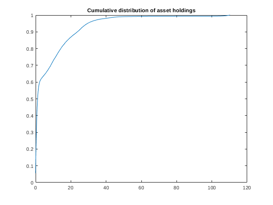
Calculating various equilibrium objects

Display some output about the solution
figure(3)
plot(a_grid,cumsum(sum(StationaryDist.ptweights(1)*StationaryDist.impatient,2)+sum(StationaryDist.ptweights(2)*StationaryDist.patient,2))) %Plot the asset cdf
title('Cumulative distribution of asset holdings')

fprintf('For parameter values sigma=%.2f, mu=%.2f, rho=%.2f \n', [Params.sigma,Params.mu,Params.rho])

fprintf('The equilibrium value of the interest rate is r=%.4f \n', p_eqm.r*100)
fprintf('The equilibrium value of the aggregate savings rate is s=%.4f \n', aggsavingsrate)
%fprintf('Time required to find the eqm was %.4f seconds \n',findeqmtime)
For parameter values sigma=0.20, mu=3.00, rho=0.60 
The equilibrium value of the interest rate is r=2.0188 
The equilibrium value of the aggregate savings rate is s=0.2915 
 

Published with MATLAB® R2018a